Download
1 / 44
440 likes | 443 Views
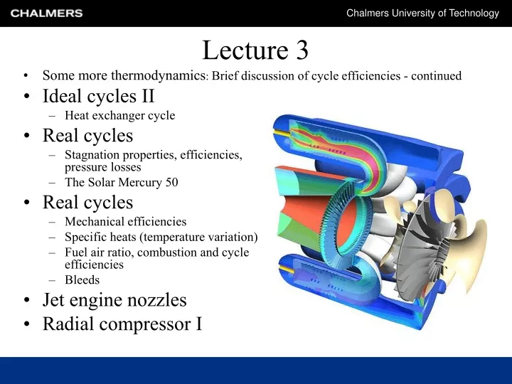
Lecture 3. Some more thermodynamics : Brief discussion of cycle efficiencies - continued Ideal cycles II Heat exchanger cycle Real cycles Stagnation properties, efficiencies, pressure losses The Solar Mercury 50 Real cycles Mechanical efficiencies Specific heats (temperature variation)

E N D
Lecture 3 Some more thermodynamics: Brief discussion of cycle efficiencies - continued Ideal cycles II Heat exchanger cycle Real cycles Stagnation properties, efficiencies, pressure losses The Solar Mercury 50 Real cycles Mechanical efficiencies Specific heats (temperature variation) Fuel air ratio, combustion and cycle efficiencies Bleeds Jet engine nozzles Radial compressor I
Generalization of the Carnot efficiency Is generalization of Carnot efficiencyto Brayton cycle possible? Define average temp. to value that would give the same heat transfer, i.e.:
Generalization of Carnot efficiency But for the isobar we have, Furthermore, we have Gibbs equation (Cengel and Boles): as well as: Thus, the average temperature is obtained from (dp=0): Derive an expression for the lower average temperature in the same way.
Heat exchange cycle When T4 > T2 a heat exchanger can be introduced. This is true when:
Theory 3.1 – Ideal heat exchanger cycle Here we obtain the efficiency: Not independent of T3!!! (simple cycle is independent of t3) Power output is unaffected by heat exchangers since the turbine and compressor work are the same as in the simple cycle.
Heat exchange cycle Very high efficiencies can be theoretically be obtained! Heat exchanger metallurgical limits will be relevant. T4 = 1000.0 K =>
Heat exchange cycle What happens with the average temperature at which heat is added/rejected when the pressure ratio changes in heatexchange cycle? TH TH qin qin qout qout Low pressure ratio=> high efficiency
Cycles with losses • Change in kinetic energy between inlet and outlet may not be negligible : • Fluid friction => - burners - combustion chambers - exhaust ducts
Heat exchangers. Economic size => terminal temperature difference, i.e. T5 < T4. Friction losses in shaft, i.e. the transmission of turbine power to compressor. Auxiliary power requirement such as oil and fuel pumps. γ and cp vary with temperature and gas composition. Cycles with losses
Efficiency is defined by SFC (specific fuel consumption = fuel consumption per unit net work output). Cycle efficiency obtained using fuel heating value. Cooling of blade roots and turbine disks often require approximately the same mass flow of gas as fuel flow => air flow is approximated as constantfor preliminary calculations. Thisis done in this course. Cycles with losses
Stagnation properties • For high-speed flows, the potential energy of the fluid can still be neglected but the kinetic energy can not! • It is convenient to combine the static temperature and the kinetic energy into a single term called the stagnation (or total) enthalpy, h0=h+V2/2, i.e. the energy obtained when a gas is brought to rest without heat or work transfer
Stagnation properties For a perfect gas we get the stagnation temperature T0, according to:
Stagnation pressure • Defined in same manner as stagnation temperature (no heat or work transfer) with added restriction • retardation is thought to occur reversibly • Thus we define the stagnation pressure p0 by: • Note that for an isentropicprocess between 02 and 01 we get
Compressor and turbine efficiencies Isentropic efficiency (compressors and turbines are approximately adiabatic => if expansion is reversible it is isentropic). The isentropic efficiency is for the compressor is: Where are the averaged specific heats of the temperature intervals 01-02´ and 01-02 respectively.
Compressor and turbine efficiencies • Similarly for the turbine: • Ideal and mean temperature differences are not very different. Thus it is a good approximation to assume: • We therefore define:
Compressor and turbine efficiencies Using produces the frequently used expressions:
Turbine efficiency options • If the turbine exhausts directly to atmosphere the kinetic energy is lost and a more proper definition of efficiency would be: • In practice some of the kinetic energy is recovered in an exhaust diffuser => turbine pressure ratio increases. • Here we put p04=pa for gas turbines exhausting into atmosphere and think of ηt as taking both turbine and exhaust duct losses into account
Turbine diffusers Recovered energy
Heat-exchanger efficiency Conservation of energy (neglecting energy transfer to surrounding): In a real heat-exchanger T05 will no longer equal T04 (T05 <T04). We introduce heat exchanger effectiveness as: • Modern heat exchangers are designed to for effectiveness values above 90%. Use of stainless steel requires T04 around 900 K (or less). More advanced steal alloys can be used up to 1025 K.
Pressure losses – burners & heat-exchangers • Burner pressure losses • Flame stabilizing & mixing • Fundamental loss (Chapter 7 + Rayleigh-line appendix A.4) • Heat exchanger pressure loss • Air passage pressure loss ΔPha • Gas passage pressure loss ΔPhg • Losses depend on heat exchanger effectiveness. A 4% pressure loss is a reasonable starting point for design.
The Solar Mercury 50 • 4.3 MW output • η = 40.5 % • System was designed from scratch to allow high performance • integration of heat-exchanger
Mechanical losses Turbine power is transmitted directly from the turbine without intermediate gearing => (only bearing and windage losses). We define the transmission efficiency ηm: Usually power to drive fuel and oil pumps are transmitted from the shaft. We will assume ηm=0.99 for calculations.
We have already established: cp=f1(T) cv=f2(T) Since γ =cp/cv we have γ=f3(T) The combustion product thermodynamic properties will depend on T and f (fuel air ratio) Temperature variation of specific heat
Pressure dependency? At 1500 K dissociation begins to have an impact on cp and γ. Detailed gas tables for afterburners may include pressure effects. We exclude them in this course.
Temperature variation of specific heat In this course we use: Since gamma and cp vary in opposing senses some of the error introduced by this approximation is cancelled.
Determining the fuel air ratio Calculate f that gives T03 for given T02? Use first law for control volumes (q=w=0) and that enthalpy is a point function (any path will produce the same result) f is small (typically around 0.02) and cpf is also small => last term is negligible. The equation determines f.
Combustion temperature rise Hypothetic fuel: 86.08% carbon 13.92% hydrogen ΔH25 = - 43100 kj/kg Curves ok for kerosene burned in dry air. Not ok in afterburner (fin≠0).
Combustor and turbine regions require most of the cooling air. Anti-ice Rule of thumb: take air as early as possible (less work put in) Accessory unit cooling (oil system, aircraft power supply (generator), fuel pumps) Air entering before rotor contributes to work! Bleeds
Jet engine – principles of thrust generation No heat or work transfer in the jet engine nozzle Stagnation temperature is constant
Mach number relations for stagnation properties We have already introduced the stagnation temperature as: and shown that (revision task): The specific heat ratio γ is defined: The Mach number is defined as:
Mach number relations for stagnation properties Thus: but we defined: which directly gives:
Nozzle efficiencies Nozzle may operate choked or unchoked:
Nozzle efficiencies Critical pressure for irreversible nozzle is obtained from: which gives:
Basic operation of radial compressor • Impeller - work is transferred to accelerate flow and increase pressure • Diffuser - recover high speed generated in impeller as pressure
Radial compressoroperation • Typical design takes 50 % of increase in static pressure in diffuser • Conservation of angular momentum governs performance:
Slip factor Due to inertia of flow Cw2 < U: • Stanitz formula for estimating σ
Power is put into overcoming additional friction not related to the flow in the impeller channels Converts energy to heat => additional loss => Power input factor -
P03 is here used to denote the pressure at compressor exit. P02 is reserved for the stagnation pressure between the impeller and the diffuser vanes Overall pressure rise:
Example 4.1a • ψ=1.04, σ= 0.90 • N = 290.0 rev/s, • D = 0.5 m • Deye,tip = 0.3, Deye,root = 0.15 • m = 9.0 kg/s • T01 = 295 K • P01 = 1.1 bar • ηc = 0.78 • Compute pressure ratio and power required
Understand why the Carnot cycle can be used for qualitative arguments also for the Joule/Brayton cycle Be able to state reasonable loss levels for gas turbine components (turbine and compressor performance are given in Lecture 4) and include them in cycle analysis Know how to compute cycle efficiencies for the heat exchanger cycle Learning goals