Download
1 / 16
160 likes | 162 Views
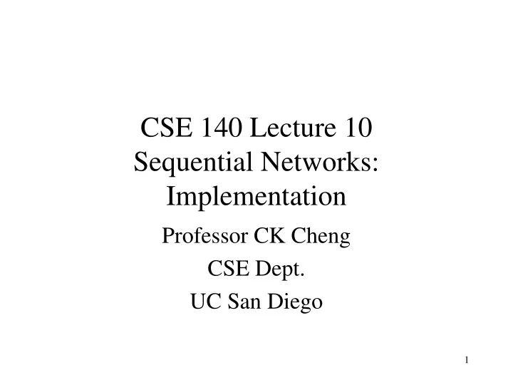
CSE 140 Lecture 10 Sequential Networks: Implementation. Professor CK Cheng CSE Dept. UC San Diego. Implementation. Format and Tool Procedure Excitation Tables Example. Canonical Form: Mealy and Moore Machines. x(t). y(t). Combinational Logic. CLK. x(t). C2. y(t). x(t). C1. C2.

E N D
CSE 140 Lecture 10Sequential Networks: Implementation Professor CK Cheng CSE Dept. UC San Diego
Implementation • Format and Tool • Procedure • Excitation Tables • Example
Canonical Form: Mealy and Moore Machines x(t) y(t) Combinational Logic CLK x(t) C2 y(t) x(t) C1 C2 y(t) C1 CLK CLK
Canonical Form: Mealy and Moore Machines Mealy Machine: yi(t) = fi(X(t), S(t)) Moore Machine: yi(t) = fi(S(t)) si(t+1) = gi(X(t), S(t)) x(t) x(t) C1 C2 y(t) C1 C2 y(t) CLK CLK s(t) s(t) Moore Machine Mealy Machine
iClicker • The advantage of Moore machine over Mealy machine is that for Moore machine, • the circuit is smaller • the circuit is faster • the input is synchronized with clock • the output is synchronized with clock • None of the above
Sequential Network Implementation:Format and Tool Canonical Form: Mealy & Moore machines State Table Netlist Tool: Excitation Table x(t) C1 C2 y(t) CLK s(t) Q(t+1) = h(x(t), Q(t)) y(t) = f(x(t), Q(t))
Implementation: Procedure Given a state table, we have NS: Q(t+1) = h(X(t),Q(t)) We want to derive D(t), T(t), (S(t) R(t)), (J(t) K(t)) as functions of (X,Q(t)). We implement D, T, (S R), (J K) as combinational logic. State Table => Excitation Table
W NS PS PS NS Implementation: Procedure F-F State Table <=> F-F Excitation Table W • W: • D F-F • D(t)= eD(Q(t+1), Q(t)) • T F-F • T(t)= eT(Q(t+1), Q(t)) • SR F-F • S(t)= eS(Q(t+1), Q(t)) • R(t)= eR(Q(t+1), Q(t)) • JK F-F • J(t)= eJ(Q(t+1), Q(t)) • K(t)= eK(Q(t+1), Q(t))
Implementation: Procedure • State table: y(t)= f(Q(t), x(t)), Q(t+1)= h(x(t),Q(t)) • Excitation table of F-Fs: • D(t)= eD(Q(t+1), Q(t)); • T(t)= eT(Q(t+1), Q(t)); • (S, R), or (J, K) • From 1 & 2, we derive excitation table of the system • D(t)= gD(Q(t), x(t))= eD(h(x(t),Q(t)),Q(t)); • T(t)= gT(Q(t), x(t))= eT(h(x(t),Q(t)),Q(t)); • (S, R) or (J, K). • Use K-map to derive optional combinational logic implementation. • T(t)= gT(Q(t), x(t)) • y(t)= f(Q(t), x(t))
JK 00 0 1 11 1 0 10 1 1 01 0 0 0 1 Q(t+1) Q(t) Q(t+1) NS PS 0 0- -1 1 1- -0 0 1 Q(t) JK Excitation Table State table of JK F-F: Excitation table of JK F-F: If Q(t) is 1, and Q(t+1) is 0, then JK needs to be 0-.
Excitation Tables and State Tables State Tables: Excitation Tables: SR SR Q(t+1) NS SR PS PS 0 0- 01 1 10 -0 00 0 1 01 0 0 10 1 1 11 - - 0 1 0 1 Q(t) Q(t) Q(t+1) T T Q(t+1) NS T PS PS 0 0 1 1 1 0 0 0 1 1 1 0 0 1 0 1 Q(t) Q(t) Q(t+1)
Excitation Tables and State Tables Excitation Tables: State Tables: JK JK Q(t+1) NS JK PS PS 0 0- -1 1 1- -0 00 0 1 01 0 0 10 1 1 11 1 0 0 1 0 1 Q(t) Q(t) Q(t+1) D D Q(t+1) NS D PS PS 0 0 0 1 1 1 0 0 0 1 1 1 0 1 0 1 Q(t) Q(t) Q(t+1)
iClicker • Given a flip-flop, the relation of its state table and excitation table is • One to one • One to many • Many to one • Many to many • None of the above
J Q Q’ K C1 T Implementation: ExampleImplement a JK F-F with a T F-F Q(t+1) = h(J(t),K(t),Q(t)) = J(t)Q’(t)+K’(t)Q(t) State Table JK JK PS 00 0 1 01 0 0 10 1 1 11 1 0 0 1 Q(t)
Example: Implement a JK flip-flop using a T flip-flop Excitation Table of T Flip-Flop T(t) = Q(t) XOR Q(t+1) Q(t+1) NS PS 0 0 1 1 1 0 0 1 Q(t) T Excitation Table of the Design id 0 1 2 3 4 5 6 7 J(t) 0 0 0 0 1 1 1 1 K(t) 0 0 1 1 0 0 1 1 Q(t) 0 1 0 1 0 1 0 1 Q(t+1) 0 1 0 0 1 1 1 0 T(t) 0 0 0 1 1 0 1 1 T(t) = Q(t) XOR ( J(t)Q’(t) + K’(t)Q(t))
Example: Implement a JK flip-flop using a T flip-flop T(J,K,Q): K 0 2 6 4 0 0 1 1 T = K(t)Q(t) + J(t)Q’(t) 1 3 7 5 Q(t) 0 1 1 0 J J Q Q’ T K