Download

1 / 13
130 likes | 403 Views
Evaluating Different Solution Methods for Pm|prec|C max. Jonathan Chan . Introduction. Scheduling problems of type Pm|prec|C max that are easily solvable Infinite machines : P∞|p j =1,prec|Cmax Intree, outtree precedence : Pm|p j =1,intree|C max & Pm|p j =1,outtree|C max

E N D
Evaluating Different Solution Methods for Pm|prec|Cmax Jonathan Chan
Introduction • Scheduling problems of type Pm|prec|Cmax that are easily solvable • Infinite machines: P∞|pj=1,prec|Cmax • Intree, outtree precedence: Pm|pj=1,intree|Cmax & Pm|pj=1,outtree|Cmax • However, Pm|prec|Cmax is NP-hard for 2≤m <n
3 Solution Methods • Critical path rule (CP rule) • Gives the highest priority to the job at the head of the longest string of jobs in the precedence graph • Largest Number of Successors (LNS rule) • Job with the largest total number of successors in the precedence constraints graph takes the highest priority • Fujii, Kasami, Ninomiya algorithm • Matching problem- find the maximum number of disjoint compatible task pairs
1 2 3 4 5 6 7 8 9 10 Example 1 • Consider P2| prec, pj =1| Cmax with 10 jobs • BOTH CP and LNS achieve the optimal schedule Critical Path: Cmax = 5 Largest Number of Successors: Cmax = 5
1 2 4 5 6 3 7 8 Example 2 • Consider P2| prec, pj =1 | Cmax with 8 jobs. All jobs have unit processing times. • LNS achieves the optimal schedule Critical Path Solution: Cmax = 5 Largest Number of Successors: Cmax = 4
1 2 3 4 5 6 Example 3 • Consider P2| prec | Cmax with 6 jobs. All jobs have unit processing times. • CP achieves the optimal schedule Critical Path Solution: Cmax = 3 Largest Number of Successors: Cmax = 4
Fujii, Kasami, Ninomiya algorithm • Optimal Sequencing of Two Equivalent Processors by Fujii, Kasami, Ninomiya • Algorithm for solving P2|prec, pj=1|Cmax in O(n3) time for any arbitrary precedence constraint • Step1: Find all disjoint compatible task pairs by constructing a graph Gj consisting of n vertices, where two vertices i and j are connected by an edge if there does not exist a path from i and j • Step 2: Determine the maximum set of edges such that no two contain the same vertices • Step 3: Schedule each job pair in order of their precedence relations
1 3 5 6 2 4 Applying the Algorithm • Step 1: Construct the disjoint compatible task pair graph Gj Precedence Graph Graph Gj
Applying the Algorithm • Step 2: Let A1 be the max set of disjoint compatible task pairs, and A2 be the set of remaining tasks A1= {(T3, T5), (T1, T6), (T2,T4)} A2= {0}
Applying the Algorithm Step 3: Basically schedule each job pair in order of their precedence relations, where β1, …βn-m is the optimal sequence such that βi is either a single task or task pair j =1 S1 = {T1, T2, T3, T4, T5, T6} M1=A1 = {(T3, T5), (T1, T6), (T2,T4)} β1 = (T1, T6) j=2 S2 = { T2, T3, T4, T5} M2 = {(T3, T5), (T2,T4)} β2= (T2,T4) j=3 S3= {T3, T5} M3= {(T3, T5)} β 3= (T3, T5)
1 2 3 4 5 6 Discussion of the Algorithm • Marc T. Kaufman disproves this claim that the algorithm can be applied to 3 processors • Counterexample: P3|prec, pj =1| Cmax • The max set of disjoint compatible task pairs is {T1, T5, T6} , {T4, T2, T3}, suggesting that Cmax =2. However, the optimal schedule is actually Cmax=3, and the optimal partition is {T1, T4} , {T2, T3, T5}, {T6}
Further Discussion • The quality of the solution methods, as you increase the number of machines, depends on the type of precedence constraints
Further Discussion • Example of P4|prec, pj=1|Cmax • CP Rule: Cmax = 4 • LNS Rule: Cmax = 4 • Optimal: Cmax =3 • Observation: if the number of nodes without any predecessors is less than the number of processors, then the CP rule and LNS rule will achieve the optimal schedule