Marc Moonen Dept. E.E./ESAT-STADIUS, KU Leuven marc.moonen@esat.kuleuven.be

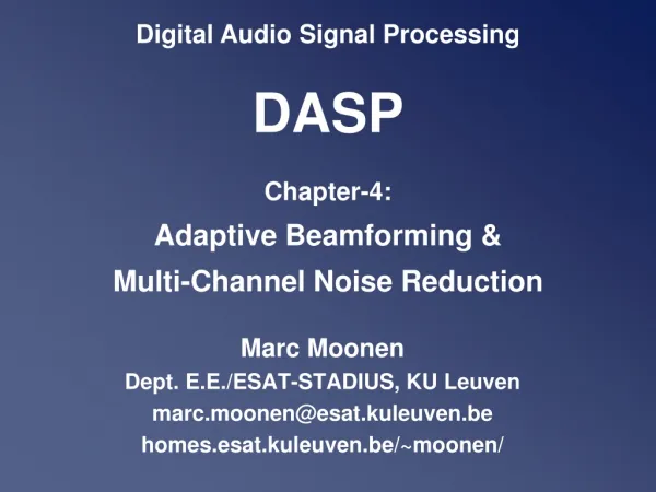
Digital Audio Signal Processing Lecture-3: Microphone Array Processing- Adaptive Beamforming - Marc Moonen Dept. E.E./ESAT-STADIUS, KU Leuven marc.moonen@esat.kuleuven.be homes.esat.kuleuven.be/~moonen/

Overview Lecture 2 • Introduction & beamforming basics • Fixed beamforming Lecture 3: Adaptive beamforming • Introduction • Review of “Optimal & Adaptive Filters” • LCMV beamforming • Frost beamforming • Generalized sidelobe canceler

Introduction Beamforming = `Spatial filtering’ based on microphone directivity patterns and microphone array configuration Classification • Fixed beamforming: data-independent, fixed filters Fm Example:delay-and-sum, filter-and-sum • Adaptive beamforming: data-dependent adaptive filters Fm Example: LCMV-beamformer, Generalized SidelobeCanceler + :

Introduction Data model& definitions • Microphone signals • Output signal after `filter-and-sum’ is • Array directivity pattern • Array gain =improvement in SNRfor source at angle 

Optimal & Adaptive Filters Review 1/6

Optimal & Adaptive Filters Review 2/6 Norbert Wiener

Optimal & Adaptive Filters Review 5/6 (Widrow 1965 !!)

LCMV-beamforming • Adaptive filter-and-sum structure: • Aim is to minimize noise output power, while maintaining a chosen response in a given look direction (and/or other linear constraints, see below). • This is similar to operation of a superdirective array (in diffuse noise), or delay-and-sum (in white noise), cfr (**) Lecture 2 p.21&29, but now noise field is unknown ! • Implemented as adaptive FIR filter : + :

LCMV-beamforming LCMV = Linearly Constrained Minimum Variance • f designed to minimize power (variance) of totaloutput(read on..) z[k] : • To avoid desired signal cancellation, add (J) linear constraints • Example: fix array response in look-direction ψ for sample freqswi, i=1..J (**)

LCMV-beamforming LCMV = Linearly Constrained Minimum Variance • With (**) (for sufficiently large J) constrained total output power minimization approximately corresponds to constrained output noise power minimization (why?) • Solution is (obtained using Lagrange-multipliers, etc..):

Frost Beamforming Frost-beamformer = adaptive version of LCMV-beamformer • If Ryy is known, a gradient-descent procedure for LCMV is : in each iteration filters f are updated in the direction of the constrained gradient. The P and B are such that f[k+1] statisfies the constraints (verify!). The mu is a step size parameter (to be tuned

Frost Beamforming Frost-beamformer = adaptive version of LCMV-beamformer • If Ryy is unknown, an instantaneous (stochastic) approximation may be substituted, leading to a constrained LMS-algorithm: (compare to LMS formula)

Generalized Sidelobe Canceler (GSC) GSC = alternative adaptive filter formulation of the LCMV-problem : constrained optimisation is reformulated as a constraint pre-processing, followed by an unconstrained optimisation, leading to a simpler adaptation scheme • LCMV-problemis • Define `blocking matrix’ Ca, ,with columns spanning the null-space of C • Define ‘quiescent response vector’ fqsatisfying constraints • Parametrize all f’s that satisfy constraints (verify!) I.e. filter f can be decomposed in a fixed part fq and a variable part Ca. fa

Generalized Sidelobe Canceler (GSC) GSC = alternative adaptive filter formulation of the LCMV-problem : constrained optimisation is reformulated as a constraint pre-processing, followed by an unconstrained optimisation, leading to a simpler adaptation scheme • LCMV-problemis • Unconstrained optimization of fa: (MN-J coefficients)

Generalized Sidelobe Canceler GSC (continued) • Hence unconstrained optimization of fa can be implemented as an adaptive filter (adaptive linear combiner), with filter inputs (=‘left- hand sides’) equal to and desired filter output (=‘right-hand side’) equal to • LMS algorithm :

Generalized Sidelobe Canceler GSC then consists of three parts: • Fixed beamformer(cfr.fq ), satisfying constraints but not yet minimum variance), creating `speech reference’ • Blocking matrix (cfr. Ca), placing spatial nulls in the direction of the speech source (at sampling frequencies) (cfr. C’.Ca=0), creating `noise references’ • Multi-channel adaptive filter (linear combiner) your favourite one, e.g. LMS +

y1 yM Postproc Generalized Sidelobe Canceler A popular GSC realization is as follows Note that some reorganization has been done: the blocking matrix now generates (typically) M-1 (instead of MN-J) noise references, the multichannel adaptive filter performs FIR-filtering on each noise reference (instead of merely scaling in the linear combiner). Philosophy is the same, mathematics are different (details on next slide).

Generalized Sidelobe Canceler • Math details: (for Delta’s=0) select `sparse’ blocking matrix such that : =input to multi-channel adaptive filter =use this as blocking matrix now

Generalized Sidelobe Canceler • Blocking matrix Ca (cfr. scheme page 24) • Creating (M-1) independent noise references by placing spatial nulls in look-direction • different possibilities (a la p.38) (broadside steering) Griffiths-Jim • Problems of GSC: • impossible to reduce noise from look-direction • reverberation effects cause signal leakage in noise references • adaptive filter should only be updated when no speech is present to avoid signal cancellation! Walsh

Marc Moonen Dept. E.E./ESAT-STADIUS, KU Leuven marc.moonen@esat.kuleuven.be