Download
1 / 47
470 likes | 479 Views
Population Ecology I. Attributes II.Distribution III. Population Growth – changes in size through time IV. Species Interactions V. Dynamics of Consumer-Resource Interactions VI. Competition. VI. Competition. Overview: 1. Types:

E N D
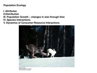
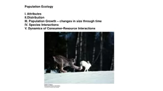
Population Ecology I. Attributes II.Distribution III. Population Growth – changes in size through time IV. Species Interactions V. Dynamics of Consumer-Resource Interactions VI. Competition
VI. Competition • Overview: • 1. Types: • - exploitative/scramble – organisms remove what they can; neither gets enough to maximize fitness
VI. Competition • Overview: • 1. Types: • - exploitative/scramble – organisms remove what they can; neither gets enough to maximize fitness • - territorial/contest/interference – competition for access to the resource, with ‘winner take all’. Winner still incurs cost of competition
VI. Competition • Overview: • 1. Types: • 2. Outcomes: • - Reduction in organism growth and/or pop. size (G, M, R) • - Competitive exclusion (N = 0) • - Change range of resources used = resource partitioning.
VI. Competition • Overview: • 1. Types: • 2. Outcomes: • - Reduction in organism growth and/or pop. size (G, M, R) • - Competitive exclusion (N = 0) • - Change range of resources used = resource partitioning. • - If this selective pressure continues, it may result in a morphological change in the competition. This adaptive response to competition is called Character Displacement
VI. Competition B. Empirical Tests of Competition 1. Gause P. aurelia vs. P. caudatum Both do well when alone, but P. aurelia outcompetes P. caudatum when together
VI. Competition B. Empirical Tests of Competition 1. Gause P. aurelia vs. P. bursaria ):
VI. Competition B. Empirical Tests of Competition 1. Gause P. aurelia vs. P. bursaria – coexist when together ):
VI. Competition B. Empirical Tests of Competition 1. Gause P. aurelia and P. caudatum feed on bacteria in the open water (same niche); P. bursaria feeds on bacteria on the glass. “Competitive exclusion principle” – Two species with the same environmental requirements (niche) cannot coexist.
VI. Competition B. Empirical Tests of Competition 1. Gause 2. Park Competition between two species of flour beetle: Tribolium castaneum and T. confusum. Tribolium castaneum
VI. Competition B. Empirical Tests of Competition 1. Gause 2. Park Competition between two species of flour beetle: Tribolium castaneum and T. confusum. Competitive outcomes are dependent on complex environmental conditions Basically, T. confusum wins when it's dry, regardless of temp.
VI. Competition B. Empirical Tests of Competition 1. Gause 2. Park Competition between two species of flour beetle: Tribolium castaneum and T. confusum. Competitive outcomes are dependent on complex environmental conditions But when it's moist, outcome depends on temperature
VI. Competition B. Empirical Tests of Competition 1. Gause 2. Park 3. Connell Intertidal organisms show a zonation pattern... those that can tolerate more desiccation occur higher in the intertidal.
3. Connell - reciprocal transplant experiments Fundamental Niches defined by physiological tolerances ): increasing desiccation stress
3. Connell - reciprocal transplant experiments Realized Niches defined by competition ): Balanus competitively excludes Chthamalus from the "best" habitat, and limits it to more stressful habitat
VI. Competition B. Empirical Tests of Competition 1. Gause 2. Park 3. Connell 4. Emery et al. (2001)
4. Emery et al. (2001) Add nutrients and the more salt tolerant species, which was competitively excluded from more benign habitats under lower nutrient conditions, now expands – nutrient limitation is relieved and the tolerant species wins.
VI. Competition C. Modeling Competition 1. Intraspecific competition The logistic curve describes intraspecific competition.
VI. Competition C. Modeling Competition 1. Intraspecific competition 2. Interspecific competition – Lotka-Volterra Models The effect of 10 individuals of species 2 on species 1, in terms of 1, requires a "conversion term" called a competition coefficient (α). So, here, 10 N2 individuals exert as much competitive stress on N1 as 20 N1 individuals…so α = 2.0 and N1 equilibrates at K – 20.
VI. Competition C. Modeling Competition 1. Intraspecific competition 2. Interspecific competition – Lotka-Volterra Models We can create an "isocline" that described the effect of species 2 on the abundance of species 1 across all abundances of species 2. For example, as we just showed, 10 individuals of species 2 reduces species 1 by 20 individuals, so species 1 will equilibrate at N1 = 60.
VI. Competition C. Modeling Competition 1. Intraspecific competition 2. Interspecific competition – Lotka-Volterra Models and when N2 = 20 (exerting a competitive effect equal to 40 N1 individuals), then N1 will equilibrate at N1 = 40.
VI. Competition C. Modeling Competition 1. Intraspecific competition 2. Interspecific competition – Lotka-Volterra Models And, when species 2 reaches an abundance of 40 (N2 = K1/α12) it drives species 1 from the environment (competitive exclusion). In this case, species 1 equilibrates at N1 = 0. So, this line describes the density at which N1 will equilibrate given a particular number of N2 competitors in the environment. This is the isocline describing dN/dt = 0.
VI. Competition C. Modeling Competition 1. Intraspecific competition 2. Interspecific competition – Lotka-Volterra Models Generalized isocline for species 1.
VI. Competition C. Modeling Competition 1. Intraspecific competition 2. Interspecific competition – Lotka-Volterra Models And for two competing species, describing their effects on one another.
VI. Competition C. Modeling Competition 1. Intraspecific competition 2. Interspecific competition – Lotka-Volterra Models Now, if we put these isocline together, we can describe the possible outcomes of pairwise competition. If the isoclines align like this, then species 1 always wins.We hit species 2's isocline first, and then as abundances increase, species 2 must decline while species 1 can continue to increase. Eventually, species 2 will be driven to extinction and species 1 will increase to its carrying capacity.
VI. Competition C. Modeling Competition 1. Intraspecific competition 2. Interspecific competition – Lotka-Volterra Models Now, if we put these isocline together, we can describe the possible outcomes of pairwise competition. If the isoclines align like this, then species 2 always wins. We hit species 1's isocline first, and then as abundances increase, species 1 must decline while species 1 can continue to increase. Eventually, species 1 will be driven to extinction and species 2 will increase to its carrying capacity.
VI. Competition C. Modeling Competition 1. Intraspecific competition 2. Interspecific competition – Lotka-Volterra Models Now, if we put these isocline together, we can describe the possible outcomes of pairwise competition. The effects are more interesting if the isoclines cross. There is now a point of intersection, where BOTH populations have a non-zero equilibrium. This is competitive coexistence. Here it is stable - a departure from this point drives the dynamics back to this point. Essentially, each species reaches it's own carrying capacity before it can reach a density at which it would exclude the other species.
VI. Competition C. Modeling Competition 1. Intraspecific competition 2. Interspecific competition – Lotka-Volterra Models Now, if we put these isocline together, we can describe the possible outcomes of pairwise competition. Here the isocline cross, too. But each species reaches a density at which it would exclude the other species before it reaches its own carrying capacity. So, although an equilibrium is possible (intersection), it is unstable... any deviation will result in the eventual exclusion of one species or the other.
VI. Competition C. Modeling Competition 1. Intraspecific Competition 2. Interspecific Competition – Lotka-Volterra Models - need to do a competition experiment first, to measure α’s, to predict outcomes of other competition experiments - don’t know anything about the nature of the competitive interaction… what are they competing for?
VI. Competition C. Modeling Competition 1. Intraspecific Competition 2. Interspecific Competition – Lotka-Volterra Models 3. Tilman’s Resource Models (1982) ):
3.Tilman's Resource Models (1982) Isoclines graph population growth relative to resource ratios (2 resources, R1, R2) CA = Consumption rate of sp. A. ): So, species A consumes 3 units of resource 2 for every unit of resource 1.
3.Tilman's Resource Models (1982) Isoclines graph population growth relative to resource ratios (2 resources, R1, R2) CA = Consumption rate of sp. A. ): So, species A consumes 3 units of resource 2 for every unit of resource 1. BUT: It needs more resource 2; it can by on a small amount of resource 1.
3. Tilman's Resource Models (1982) Isoclines graph population growth relative to resource ratios (2 resources, R1, R2) CA = Consumption rate of Sp. A. Resource limitation can occur in different environments with different initial resource concentrations (S1, S2). So, in S2, the population becomes limited by the lower supply of R2. The lower supply of R1 in S1 is not a problem because the species uses this resource so slowly. ):
Species B requires more of both resources than species A. So, no matter the environment and no matter the consumptions curves (lines from S), the isocline for species B will be "hit" first. So, Species B will stop growing, but Species A can continue to grow and use up resources.... this drops resources below B's isocline, and B will decline.
Species B requires more of both resources than species A. So, no matter the environment and no matter the consumptions curves (lines from S), the isocline for species B will be "hit" first. So, Species B will stop growing, but Species A can continue to grow and use up resources.... this drops resources below B's isocline, and B will decline. So, if one isocline is completely within the other, then one species will always win.
If the isoclines intersect, coexistence is possible (there are densities where both species are equilibrating at values > 1).
If the isoclines intersect, coexistence is possible (there are densities where both species are equilibrating at values > 1). Whether this is a stable coexistence or not depends on the consumption curves. Consider Species B. It requires more of resource 1, but less of resource 2, than species A. Yet, it also consumes more of resource 1 than resource 2 - it is a "steep" consumption curve. So, species B will limit its own growth more than it will limit species A.
If the isoclines intersect, coexistence is possible (there are densities where both species are equilibrating at values > 1). Whether this is a stable coexistence or not depends on the consumption curves. Consider Species B. It requires more of resource 1, but less of resource 2, than species A. Yet, it also consumes more of resource 1 than resource 2 - it is a "steep" consumption curve. So, species B will limit its own growth more than it will limit species A. This will be a stable coexistence for environments with initial conditions between the consumption curves (S3). If the consumption curves were reversed, there would be an unstable coexistence in this region.
3. Tilman's Resource Models (1982) - Benefits: 1. The competition for resources is defined
3. Tilman's Resource Models (1982) - Benefits: 1. The competition for resources is defined 2. The model has been tested in plants and plankton and confirmed
3. Tilman's Resource Models (1982) - Benefits: 1. The competition for resources is defined 2. The model has been tested in plankton and confirmed Cyclotella wins Cyclotella Stable Coexistence Asterionella wins PO4 (uM) Asterionella SiO2 (uM)
3. Tilman's Resource Models (1982) - Benefits: 1. The competition for resources is defined 2. The model has been tested in plants and plankton and confirmed 3. Also explains an unusual pattern called the "paradox of enrichment"
3. Tilman's Resource Models (1982) - Benefits: 1. The competition for resources is defined 2. The model has been tested in plants and plankton and confirmed 3. Also explains an unusual pattern called the "paradox of enrichment" If you add nutrients, sometimes the diversity in a system drops... and one species comes to dominate. (Fertilize your lawn so that grasses will dominate... huh?)
If you add nutrients, sometimes the diversity in a system drops... and one species comes to dominate. Change from an initial stable coexistence scenario (S1) to a scenario where species A dominates (S2).