Download
1 / 26
260 likes | 273 Views
Inference for Simple Regression. Social Research Methods 2109 & 6507 Spring 2006 March 15, 16, 2006. Regression Equation. Equation of a regression line: (y_hat) = α +βx y = α +βx + ε y = dependent variable x = independent variable

E N D
Inference for Simple Regression Social Research Methods 2109 & 6507 Spring 2006 March 15, 16, 2006
Regression Equation Equation of a regression line: (y_hat) = α +βx y = α +βx + ε y = dependent variable x = independent variable β = slope = predicted change in y with a one unit change in x α= intercept = predicted value of y when x is 0 y_hat = predicted value of dependent variable
補充: Proportional Reduction of Error (PRE)(消減錯誤的比例) • PRE measures compare the errors of predictions under different prediction rules; contrasts a naïve to sophisticated rule • R2 is a PRE measure • Naïve rule = predict y_bar • Sophisticated rule = predict y_hat • R2 measures reduction in predictive error from using regression predictions as contrasted to predicting the mean of y
Example: SPSS Regression Procedures and Output • To get a scatterplot (): 統計圖(G) → 散佈圖(S) →簡單 →定義(選x及y) • To get a correlation coefficient: 分析(A) → 相關(C) → 雙變量 • To perform simple regression 分析(A) → 回歸方法(R) → 線性(L) (選x及y)(還可選擇儲存預測值及殘差)
SPSS Example: Infant mortality vs. Female Literacy, 1995 UN Data
Example: correlation between infant mortality and female literacy
Regression: infant mortality vs. female literacy, 1995 UN Data
Global test--F檢定: 檢定迴歸方程式有無解釋能力 (β= 0)
The regression model (迴歸模型) • Note: the slope and intercept of the regression line are statistics (i.e., from the sample data). • To do inference, we have to think of α and β as estimates of unknown parameters.
Regression as conditional means • Ways to think about regression: • Straight-line description of association • Prediction • Conditional means (條件平均數) Conditional mean: a mean computed conditional on the value of another variable Regression line predicts the conditional mean of y given x
Assumptions for regression inference Think about there as being a population or “true” regression line Assumptions: • For any fixed value of x, the response (y) varies according to a normal distribution. Repeated responses y are independent of each other. • μy = α +βx (means of y conditional on x fall in a straight line) • The standard deviation of y (call it σ) for each value of x is the same. The value of σ is unknown.
Inference for regression • Population regression line: μy = α +βx estimated from sample: (y_hat) = a + bx b is an unbiased estimator (不偏估計式)of the true slope β, and a is an unbiased estimator of the true intercept α
Sampling distribution of a (intercept) and b (slope) • Mean of the sampling distribution of a is α • Mean of the sampling distribution of b is β
Sampling distribution of a (intercept) and b (slope) • Mean of the sampling distribution of a is α • Mean of the sampling distribution of b is β • The standard error of a and b are related to the amount of spread about the regression line (σ) • Normal sampling distributions; with σ estimated use t-distribution for inference
The standard error of the least-squares line • Estimate σ (spread about the regression line using residuals from the regression) • recall that residual = (y –y_hat) • Estimate the population standard deviation about the regression line (σ) using the sample estimates
Standard Error of Slope (b) • The standard error of the slope has a sampling distribution given by: • Small standard errors of b means our estimate of b is a precise estimate of • SEb is directly related to s; inversely related to sample size (n) and Sx
Confidence Interval for regression slope A level C confidence interval for the slope of “true” regression line β is b ± t * SEb Where t* is the upper (1-C)/2 critical value from the t distribution with n-2 degrees of freedom To test the hypothesis H0: β= 0, compute the t statistic: t = b/ SEb In terms of a random variable having the t,n-2 distribution
Significance Tests for the slope Test hypotheses about the slope of β. Usually: H0: β= 0 (no linear relationship between the independent and dependent variable) Alternatives: HA: β> 0 or HA: β< 0 or HA: β ≠ 0
Statistical inference for intercept We could also do statistical inference for the regression intercept, α Possible hypotheses: H0: α = 0 HA: α≠ 0 t-test based on a, very similar to prior t-tests we have done For most substantive applications, interested in slope (β), not usually interested in α
Regression: infant mortality vs. female literacy, 1995 UN Data
Hypothesis test example 大華正在分析教育成就的世代差異,他蒐集到117組父子教育程度的資料。父親的教育程度是自變項,兒子的教育程度是依變項。他的迴歸公式是:y_hat = 0.2915*x +10.25 迴歸斜率的標準誤差(standard error)是: 0.10 • 在α=0.05,大華可得出父親與兒子的教育程度是有關連的嗎? • 對所有父親的教育程度是大學畢業的男孩而言,這些男孩的平均教育程度預測值是多少? • 有一男孩的父親教育程度是大學畢業,預測這男孩將來的教育程度會是多少?