Download
1 / 30
300 likes | 318 Views
THERMOMECHANICAL ANALYSIS OF THE MAGNETIC HORN. Cracow University of Technology Institute of Applied Mechanics. P. Cupial with the contribution by Adam Wroblewski. EURO Project, WP-2. Aim and outline of the talk.

E N D
THERMOMECHANICAL ANALYSIS OF THE MAGNETIC HORN Cracow University of Technology Institute of Applied Mechanics P. Cupial with the contribution by Adam Wroblewski EURO Project, WP-2
Aim and outline of the talk The aim is to make the assessment of the horn temperature and the dynamic stress levels due to secondary particles, a step in the design of the integrated target-horn system. • Horn geometry and approximate heat sources due to secondary particles • Finite element model of the horn • Steady-state analytical vs. finite element calculations of water cooling (A.Wroblewski) • Finite-element results of temperature distribution in a horn subjected to secondary-particle heating and water cooling (A.Wroblewski) • Thermomechanical transient analysis of the horn due to thermal pulses from secondary particles • Analysis of the stresses due to current pulses in the horn • Conclusions
48.2 kW 67kW 14.9kW 78.7kW +8kW from Joule effect Energy deposition due to secondary particles 4MW, 2.2 GeV proton beam • Main assumptions: • The power dissipated is for a 4MW, 2.2 GeV proton beam and has been taken from the available sources and will be updated during the design stage when more detailed data are availabe for the Superbeam horn (recent study by C. Bobeth) • It is assumed that the power dissipated has a uniform density. Localized power release (e.g. highly non-uniform through-thickness distribution) will effect significantly the results
Z Y X Finite-element model of the horn
Steady-state temperature calculation with a simpified model • Assumptions: • Temperatures do not vary over the thickness of each cylinder wall and over water channel • thickness • All heat generated is applied only within the • thicker of the two cylinders 4 unknowns: x=Q1/Q2, Tw2, Ts1, Ts2 • Global heat balance • Heat balance in water channel • Convection conditions on the interfaces between thick wall and water as well as between thin wall and air (in the presence of turbulent flow) • 4. Spray conditions 4 non-linear equations
Temperature distribution – comparison between analytical-, Fluent and Ansys results Temperature in K for a smooth pipe Corrugated profile increases effectiveness thanks to increased wetted surface Smooth pipe Corrugated pipe
Comments on different approaches used • Good agreement has been achieved between the temperatures calculated by the three analysis methods used in the case of the smooth profile. • Standard turbulence model (one used in calculations) in Fluent loses convergence at very high Reynolds numbers (Re>10000). Ansys has been found to be more stable and therefore it has been used in the analysis of the complete horn. • Simplified engineering calculations give good estimates for a smooth cylindrical surface, but are less accurate for corrugated surfaces or for the conical geometry. • The simplified calculations provide no information on the pressure drop and flow resistance.
Temperature distribution for the one-horn configuration Temperature and water flow rate distributions in the horn for the specified energy deposition. The case of one horn with 4MW beam power. Maximum temperature of 446 K exceeds the design value for aluminium Maximum allowable water flow velocity in the water channel is taken to be 1 m/s (as recommended for heat exchengers)
The effect of increasing the flow rate twice The maximum temperature on the horn goes down to 359 K The flow rate now is locally 2.6 m/s. This flow rate is higher than the value recommended for flows in heat exchangers. It is possible to obtain the necessary flow rate by increasing the water channel gap (for this study it was assumed to be 2 mm)
Temperature distribution for a configuration with four horns Maximum temperature is 340 K for the flow velocity of 1 m/s – this is acceptable for the present design, but no heat from the target has been taken into account. The efficiency of the target cooling system is being considered by B. Lepers
Benchmark for thermal shock calculation – a plate under a pulse of heat flux A simply-supported plate made of aluminium subjected to a pulse of heat flux applied to the top surface. Adiabatic conditions are assumed on all surfaces except the top one where heat is applied. Plate dimensions: a=0.1 m, b=0.15 m (sides), h=0.001 m (thickness).
Temperature and displacement vs. time under heat pulse – analytical solution The temperature field T(z,t) is found as a solution of the transient one-dimensional heat conduction equation: with boundary conditions: The plate deforms in bending under the applied heat flux; the displacements are the solution of the dynamic plate bending problem: - coefficient of linear thermal expansion
20 18 16 14 12 TEMPERATURE (K) 10 8 6 4 2 (x10**-2) 0 0 .4 .8 1.2 1.6 2 .2 .6 1 1.4 1.8 TIME (s) Temperature rise vs. time due to a pulse of heat flux – analytical solution vs. Ansys The plate is subjected to a rectangular pulse of 5 s duration with amplitude 4*109 W/m2. The results are shown for the point with in-plane coordinates: x=a/2, y=b/2, at a distance h/4 from the surface to which the heat pulse is applied
(x10**-3) 2.4 2 1.6 1.2 .8 DISPLACEMENT (m) .4 0 -.4 -.8 -1.2 (x10**-2) -1.6 0 .4 .8 1.2 1.6 2 .2 .6 1 1.4 1.8 TIME (s) Displacement in the benchmark problem – analytical solution vs. Ansys
(x10**4) 5000 3750 2500 1250 0 STRESS SXX (Pa) -1250 -2500 -3750 -5000 -6250 (x10**-2) -7500 0 .4 .8 1.2 1.6 2 .2 .6 1 1.4 1.8 TIME (s) (x10**4) 3000 2000 1000 0 STRESS SYY (Pa) -1000 -2000 -3000 -4000 -5000 -6000 (x10**-2) -7000 0 .4 .8 1.2 1.6 2 .2 .6 1 1.4 1.8 TIME (s) Stresses in the benchmark problem – analytical solution vs. Ansys Very good agreement has been achieved for the temperature, displacement and the stress levels
Peak power calculation during the pulse The pulse duration is 5s. Energy deposited per pulse: Power during pulse: Energy and power densities are more than ten times smaller than in the target, hence less temperature increase.
2.5 2.25 2 1.75 1.5 TEMPERATURE (K) 1.25 1 .75 .5 .25 (x10**-2) 0 0 .4 .8 1.2 1.6 2 .2 .6 1 1.4 1.8 TIME (s) Dynamic response of the horn due to a single heat pulse from secondary particles All dynamic results are discussed for the case of 4 MW proton beam. Peak power during the pulse is calculated using the distribution of the average power deposition due to secondary paticles as has been used for the steady-state study. Temperature vs. time at a selected point on the horn waist (horn cylindrical part in the direct vicinity of the target).
Z Y X MX MN .268666 .386E+07 .772E+07 .116E+08 .154E+08 .193E+07 .579E+07 .965E+07 .135E+08 .174E+08 MX Response of the horn to a pulse of secondary particles – stress levels The equivalent (von Mises) stress is locally above 10 MPa. It stays below10MPa away from the region of localized stress.
(x10**3) (x10**3) 5000 6250 3750 5000 2500 3750 1250 2500 0 AXIAL STRESS (Pa) 1250 HOOP STRESS (Pa) -1250 0 -2500 -1250 -3750 -2500 -5000 -3750 -6250 -5000 (x10**-2) -7500 (x10**-2) -6250 0 .4 .8 1.2 1.6 2 0 .4 .8 1.2 1.6 2 .2 .6 1 1.4 1.8 .2 .6 1 1.4 1.8 TIME (s) TIME (s) Response of the horn due to a single heat pulse from secondary particles Stress (axial and hoop component) vs. time at a point on the horn waist.
(x10**3) 8000 7200 6400 5600 4800 VON MISES STRESS (Pa) 4000 3200 2400 1600 800 0 (x10**-2) 0 .4 .8 1.2 1.6 2 .2 .6 1 1.4 1.8 TIME (s) Response of the horn due to a single heat pulse from secondary particles Equivalent (von Mises) stress.
Response to a sequence of twenty-five pulses Temperature vs. time due to 25 pulses repeated at 50 Hz. Adiabatic conditions have been used– no account for the heat removal by the cooling system
Response to a sequence of twenty-five pulses Axial and hoop stress at a point on the horn waist. Maximum dynamic stress levels less than 10 MPa. Impuse stress is superimposed on the quasi-static one – important in the assessment of the integrity of the horn.
Response to a sequence of twenty-five pulses Equivalent stress (von Mises stress). The maximum value for 25 pulses goes up to 11 MPa. The steady-state quasi static stress level is governed by the cooling system performance and can be determined from the steady-state analysis.
Z Y X -493180 -383585 -273989 -164393 -54798 -438383 -328787 -219191 -109596 0 Horn response to a current pulse The horn is subjected to half-sine current pulses of amplitude 300 kA of 100s duration. The efect of current pulse can be reduced to magnetic pressure acting on the horn surface using the formula (P. Wertelaers, CERN-EP/99-135): Magnetic pressure has been applied only to the horn inner conductor where it has the greatest effect. A rectangular pulse equivalent to the half-sign pulse has benn used (p above is multiplied by 2/)
Z Y X MX MX MN .001927 .352E+07 .705E+07 .106E+08 .141E+08 .176E+07 .529E+07 .881E+07 .123E+08 .159E+08 Horn response to a single current pulse Equivalent stress distribution in the horn. Maximum local stress is 16 MPa. Away from this region the stress level stays below 10 MPa.
(x10**3) (x10**4) 4800 1000 4000 800 3200 600 2400 400 1600 200 AXIAL STRESS (Pa) HOOP STRESS (Pa) 800 0 0 -200 -800 -400 -1600 -600 -2400 -800 (x10**-2) (x10**-2) -3200 -1000 0 .4 .8 1.2 1.6 2 0 .4 .8 1.2 1.6 2 .2 .6 1 1.4 1.8 .2 .6 1 1.4 1.8 TIME (s) TIME (s) Horn response to a single current pulse Stress componets vs. time at a selected point on the horn waist to a single pulse.
(x10**3) 8000 7200 6400 5600 4800 VON MISES STRESS (Pa) 4000 3200 2400 1600 800 (x10**-2) 0 0 .4 .8 1.2 1.6 2 .2 .6 1 1.4 1.8 TIME (s) Horn response to a single current pulse Von Mises stress is about 8 MPa – not high
Response to a sequence of twenty-five pulses Equivalent stress resulting from a sequence of twenty-five pulses repeated at 50 Hz. No increase in the stress level. However, if repetition rate is an exact multiple of one of the natural frequencies impulse resonance can take place
Conclusions • Finite element calculations of the horn have been done with a view to making assessments of its thermomechanical and dynamic performance. • The calculations used the energy deposition data from the literature (for a 4MW, 2.2GeV proton beam). Detailed energy deposition data are very much needed in order to update these results. • Energy from secondary particles has been assumed to be released uniformly over the horn sections. Localized power release (e.g. highly non-uniform through-thickness distribution) would substantialy effect the results discussed. • The first study of the cooling system performence shows that its design can be crucial for the integration of the horn inside the target. One concept of the cooling system has been studied and more design work is now under way. • Heating from the target has not been accounted for. This will be included in the model of the integrated system when the target cooling design is proposed (B.Lepers)
The dynamic stress levels due to energy deposition in the horn have quite acceptable levels, for the power deposition assumptions used. • The calculated stress levels are important for the assessment of the horn fatigue life (see the presentation by M.Kozien and A.Wroblewski). • The results in this presentation have demonstrated the approach we are taking to studying engineering integration issues. The results will need to be updated and at this stage they are not the design values!