Download
1 / 74
740 likes | 757 Views
Atomic Force Microscopy (AFM). Operating principle Cantilever response modes Short theory of forces Force-distance curves Operating modes contact tapping –non contact AM-AFM FM-AFM Examples. Bibliography.

E N D
Atomic Force Microscopy (AFM) • Operating principle • Cantilever response modes • Short theory of forces • Force-distance curves • Operating modes • contact • tapping –non contact • AM-AFM • FM-AFM • Examples Bibliography • Scanning Probe Microscopies: Atomic Scale Engineering by Forces and Currents • NT-MDT slides
AFM basics Basic idea: Surface-tip interaction Response of the cantilever Contact Mode Tapping Mode Non-Contact Mode
AFM basics The AFM working principle Measurement of the tip-sample interaction force Probes: elastic cantilever with a sharp tip on the end The applied force bends the cantilever By measuring the cantilever deflection it is possible to evaluate the tip–surface force. How to measure the deflection 4 quadrant photodiode
AFM basics Two force components: FZ normal to the sample surface FL In plane, cantilever torsion I01, I02, I03, I04, reference values of the photocurrent I1, I2, I3, I4, values after change of cantilever position Differential currents ΔIi= Ii - I0i will characterize the value and the direction of the cantilever bending or torsion. ΔIZ = (ΔI1 + ΔI2) − (ΔI3 + ΔI4) ΔIL = (ΔI1 + ΔI4) − (ΔI2 + ΔI3) ΔIZ is the input parameter in the feedback loop keeping ΔIZ = constant in order to make the bending ΔZ = ΔZ0 preset by the operator.
Cantilever response The tip is “in contact” with the surface Interaction forces cause the cantilever to bend while scanning l = cantilever lenght w = cantilever width t = cantilever height ltip = tip height The deflection vector is linearly dependent on applied force according to Hooke’s law
Cantilever response Vertical forces Vertical force Fz applied at the end induces the cantilever bending Consider vertical force only y = cantilever deflectionalong y z = cantilever deflectionalong z = deflection angle cantilever deflection angle around setpoint
Cantilever response Assume a bending with radius R inner edge -> compressed. Neutral axis outer edge -> stretched. dF there is a neutral plane of zero stress between the two surfaces Section the longitudinal extension L is proportional to the distance z from the neutral plane Hooke’s law Y = Young modulus Resulting force acting on dS
Cantilever response Resulting force acting on dS Section At any section S there is a torque wrt neutral axis Iz= momentum of inertia of the section wrtneutral axis u(y) = deflection along z of a cantilever point at the distance y from the fixed end The point trajectory follows a curve with curvature y For small angles
Cantilever response y For small angles For any point along the cantilever y direction integration integration
Cantilever response The deflection is proportional to measured signal The feedback keeps a constant cantilever deflection, obtaining a constant force surface image The variationin the force while scanning leads to changes in z, providing the topography. Force setpoint: the force intensity exerted by the tip on the surface when approached. ~ 0.1 nN Interatomic force constants in solids: 10 100 N/m In biological samples ~ 0.1 N/m. Typical values for k in the static mode are 0.01–5 N/m. Soft cantilever
Cantilever response coefficient of inverse stiffness The magnitude characterizes the cantilever stiffness It is the largest among the tensor cij Ltip << L so cyz can be neglected Force spectroscopy at fixed location
Cantilever response Longitudinal forces Longitudinal force Fy applied at the end induces the cantilever bending: Y-type bending z = cantilever deflection along y z = cantilever deflection along z = deflection angle Longitudinal force Fy applied at the end results in a torque cantilever deflection angle around setpoint Similarly to previous case
Cantilever response Longitudinal force Fy applied at the end induces the cantilever bending but The deflection is proportional to measured signal the axial force results in the tip deflection in vertical direction
Cantilever response Longitudinal force Fy applied at the end induces the cantilever bending From the figure Very small compared to c the axial force results in the tip deflection not only in the vertical but also in longitudinal direction All these deflections are small compared to the main bending in the z axis
Cantilever response simple bending Transverse forces Transverse force Fx The simple bending is similar to the vertical bending of z-type Exchange the beam width (w) with thickness (t) torsion
Cantilever response Torsion The torsion is directly related to beam deflecton angle G= Shear modulus ~ 3Y/8 The torque by Fx is The lateral deflection is
Cantilever response Simple bending torsion The deflections in y and z are of the second order with respect to x deflection
Cantilever response L = 90 m Ltip = 10 m w = 35 m t = 1 m Dominant distortions czz, cyz, czy Lateral distortions are much smaller
Cantilever effective mass and eigenfrequency Cantilever is vibrating along z l = cantilever lenght w = cantilever width t = cantilever height ltip = tip height Fixed end y u(y) dy u(t,y) = deflection along z of a cantilever point at the distance y from the fixed end Kinetic energy u(t,L) = deflection along z of cantilever free end
Cantilever effective mass and eigenfrequency Kinetic energy work done to move the beam end the distance u(t,L) Potential energy Equation of motion Cantilever eigenfrequency The cantilever eigenfrequency must be as high as possible to avoid excitation of natural oscillations due to the probe trace-retrace move during scanning or due to external vibrations influence
Tip-surface interaction Origin of forces Tip-surface Separation (nm) 1000 Electric, magnetic, capillary forces Non contact 100 Intermittent contact Van der Waals (Keesom,Debye,London) 10 1 Contact Interatomic forces (adhesion, Hertz problem) 0
- - + + Origin of forces Contact Cgs/esu Born repulsive interatomic forces Origin: large overlap of wavefunction of ion cores of different molecules Pauli and ionic repulsion
Origin of forces Contact Elastic forces in contact Origin: object deformation when in contact Hertz problem: determination of deformation Assumptions • Isotropic cantilever and sample twoparametersto describeelasticproperties • Y = youngmodulus • = Poisson ratio • Close to the contactpoint the undeformedsurfaces are described by two curvature radii • Deformationsare small compared to surfaces curvature radii • Twospheresr1 = r2 a2 = hR Same materials deformation and penetration • Hertz problem solution: • allows to find the contact area radius a • and penetration depth h as a function of applied force • for a surface (r’=) and a tip (r=R) • contact area radius : up to 10 nm • Penetration depth : up to 20 nm • contact pressure : up to 10 GPa. the contact pressure is higher for stiffer samples
d q- q+ Intermittent contact Origin of forces Cgs/esu Keesom Dipole forces Coulomb force between point charges Coulomb potential energy Electric field = qd = dipole moment Origin: fluctuation (~10-15 s) of the electronic clouds around a molecule Dipole formation For r >> d Potential energy of the dipole moment in an electric field E Field intensity produced by the dipole is the angle between dipole and r
1 2 d d q- q- q+ q+ Intermittent contact Origin of forces Keesom Dipole forces When two atoms or molecules interacts Potential energy of the interacting dipole moments Maximum attraction for 1= 2 = 0° Maximum repulsion for 1= 2 = 90°
Intermittent contact Origin of forces Keesom Dipole forces In a gas thermal vibrations randomly rotates dipoles while interaction potential energy aligns dipoles Total orientation potential is obtained by statistically averaging over all possible orientations of molecules pair For U << KBT Orientational interaction
d d q- q- q+ q+ Intermittent contact Origin of forces Debye Dipole forces Origin: fluctuation of the electronic clouds around a molecule dipole formation, interaction of the dipole with a polarizable atom or molecule Induced dipole moment Potential energy of the interacting dipole moments The induced dipole is “istantaneous” on time scale of molecular motion So one can average on all orientations For r >> d Induction interaction
- + Intermittent contact Origin of forces London Dipole forces Origin: fluctuation of the electronic clouds around the nucleus dipole formation with the positively charged nucleus interaction of the dipole with a polarizable atom - dipole Polarizable atom + 2 1 Potential energy of atom 1 in the field due to dipole 2 Field induced by atom 2 RMS dipole moment for fluctuating electron-nucleus The dipole formation of atom 2 is given by the polarizability Ionization energy
Origin of forces Origin Potential energy Fluctuation of the electronic clouds around a molecule. dipole formation Keesom Fluctuation of the electronic clouds around a molecule. dipole formation. interaction of the dipole with a polarizable atom or molecule Debye Fluctuation of the electronic clouds around the nucleus. dipole formation with the positive charge of nucleus. interaction of the dipole with a polarizable atom London Born Large overlap of core wavefunction of different molecules
Origin of forces van der Waals dipole forces between two molecules Total potentials between two molecules Lennard-Jones potential
Origin of forces van der Waals dipole forces between macroscopic objects Additivity: the total interaction can be obtained by summation of individual contributions. Continuous medium: the summation can be replaced by an integration over the object volumes assuming that each atom occupies a volume dV with a density ρ. Uniform material properties: ρ and C1 are uniform over the volume of the bodies. The total interaction potential between two arbitrarily shaped bodies Hamaker constant
Origin of forces The force must be calculated for each shape For a pyramidal tip at distance D from surface Hamaker constant Same role as the polarizability Depends on material and shape
Origin of forces The force must be calculated for each shape Conical probe rounded tip Conical probe Pyramidal probe Tip radius r << h For r >> h Tip radius r << h
Origin of forces Adhesion forces Middle range where attraction forces (-1/r6) and repulsive forces (1/r12) act adhesion It originates from the short-range molecular forces. two types - probe-liquid film on a surface (capillary forces) - probe-solid sample (short-rangemolecularelectrostaticforces) electrostatic forces at interface arise from the formation in a contact zone of an electric double layer Origin for metals - contact potential - states of outer electrons of a surface layer atoms - lattice defects Origin for semiconductors - surface states - impurity atoms
Origin of forces Capillary forces Cantilever in contact with a liquid film on a flat surface The film surface reshapes producing the "neck“ The water wets the cantilever surface: The water-cantilever contact (if it is hydrophilic) is energetically favored as compared to the water-air contact Similar to VdW force Consequence: hysteresis in approach/retraction
Force-distance curves How to obtain info on the sample-tip interactions? Force-distance curves The sample is ramped in Z and deflection c is measured
Force-distance curves Force-distance curves The deflection of the cantilever is obtained by the optical lever technique When the cantilever bends the reflected light-beam moves by an angle c or z PSD = position sensitive detector d = detector - cantilever distance PSD = laser spot movement High sensitivity in z is obtained by L << d Vertical resolution depends on the noise and speed of PSD time for measuring a point of the force curve t= 0.1 ms z ~ 0.01 nm B. Cappella, G. Dietler, Surface Science Reports 34 (1999) 1-104
Force-distance curves Measured quantities: Z piezo displacement, PSD i.e. I or V Must be converted to D and F The sample is ramped in Z and deflection c is measured D = Z –(c+ s) D = tip-sample distance c = cantilever deflection s = sample deformation Z = piezo displacement Force – displacement curve AFM force-displacement curve doesnotreproducetip-sample interactions, butis the result of twocontributions: the tip-sample interactionF(D) and the elastic force of the cantilever F = -kcc
H.-J. Butt et al. / Surf. Sci. Rep. 59 (2005) 1 Force-distance curves Measured quantities: Z piezo displacement, PSD i.e. I or V Must be converted to D and F D = Z –(c+ s) a) Infinitely hard material (s=0), no surface forces Linear regime D = tip-sample distance c = cantilever deflection s = sample deformation Z = piezo displacement PSD-Z curve: two linear parts zero force line defines zero deflection of the cantilever Z = 0 at the intersection point Conversion between PSD and Z c = IPSD/(IPSD/ Z) sensitivity IPSD/ Z F-D curve F(Z) = kc F(D) = k IPSD(Z)/(IPSD/Z) D=Z-c In non-contact D = Z (c = 0 so F(D)=0) In contact Z = c and D = 0 so F(D)=kc Z > 0 if surface is retracted from tip
Force-distance curves Measured quantities: Z piezo displacement, PSD i.e. I or V D = Z –(c+ s) b) Infinitely hard material (s=0) long-range exponential repulsive force Linear regime D = tip-sample distance c = cantilever deflection s = sample deformation Z = piezo displacement sensitivity IPSD/ Z from the linear part PSD-Z curve c = IPSD/(IPSD/ Z) zero force line = 0 deflection at large distance Accuracy: force curves from a large distance Apply a relatively hard force to get to linear regime The degree of extrapolation determines the error in zero distance. Z = 0 at the intersection point (extrapolated) F-D curve F(Z) = kc D=Z-c F(D) = k IPSD(Z)/(IPSD/Z) In contact Z = c and D = 0 Z > 0 if surface is retracted from tip In non-contact D = Z - c
s s Force-distance curves D = Z –(c+ s) c) Deformable materials without surface force Z > 0 if surface is retracted from tip PSD-Z curve In non-contact D = Z (c = 0) D = tip-sample distance c = cantilever deflection s = sample deformation Z = piezo displacement F=0 line If tip and/or sample deform the contact part of PSD-Z curve is not linear anymore F-D curve Hertz model: elastic tip radius R planar sample of the same material (Y) s = indentation For many inorganic solids s << c For high loads c~F/kc sensitivity IPSD/ Z from the linear part If s~ c the force curves have to be modeled to describe indentation = ‘‘soft’’ samples: cells, bubbles, drops, or microcapsules. If s 0 ‘‘zero distance’’ (Z=0) must be defined In contact the distance equals an interatomic distance But: indentation and contact area are still changing with the load It is more appropriate to use indentation rather than distance after contact the abscissa would show two parameters: D before contact and sin contact
s s Force-distance curves c) Deformable materials with surface force Tip approaching a solid surface attracted by van der Waals forces - very soft materials surface forces are a problem leading to a significant deformation even before contact At some distance the gradient of the attraction exceeds kc and the tip jumps onto the surface. - relatively hard materials Due to attractive and adhesion forces it is practically difficult to precisely determine where contact is established Adhesion forces add to the spring force and can cause an indentation In this case it is practically impossible to determine zero distance and one can only assume that the indentation caused by adhesion is negligible. B. Cappella, G. Dietler, Surface Science Reports 34 (1999) 1-104
Force-distance curves Because we measure Z = the sample and the cantilever rest position separation D = Z –(c+ s) Tip-sample force Fc = -kcc Force – displacement curve Elastic force of the cantilever for different c At each distance the cantilever deflects until Fc=F(D) so that the system is in equilibrium The equilibrium points are a, b, c The corresponding distances are not D but Z i.e. the sample and the cantilever rest position separation that are given by the intersections between lines and the horizontal axis (,,) Tip-sample interaction Lennard-Jones force, F(D)= -A/D7 + B/D13
Force-distance curves Total potential of cantilever-sample system Utot = Ucs(D) + Uc(c) + Us(s) D = Z –(c+ s) assume Ucs(D) = tip - sample interactionpotential Uc(c) = cantileverelasticpotential Us(s) = sample deformationpotential The relation between Z and c is obtained by forcing the system to be stationary And since The measured force- displacement curve can be converted into the force-distance curve
Force-distance curves two characteristic features of force-displacement curves: discontinuities BB’ and CC’ hysteresis between approach and withdrawal curve jump-to-contact jump-off-contact In the region between b' and c' each line has three intersections = three equilibrium positions. Two (between c’ and b and between b' and c) are stable One (between c and b) is unstable During approach the tip follows the trajectory from c’ to b and then "jumps" from b to b‘ During retraction, the tip follows the trajectory from b' to c and then jumps from c to c’
Force-distance curves The slope of the lines 1-3 is the elastic constant of the cantilever kc. for high kc, the unsampled stretch b-c becomes smaller, the jump-to-contact first increases with kc and then, for high kc, disappears. The jump-off-contact always decreases, so that the total hysteresis diminishes with kc. When kc is greater than the greatest value of the tip-sample force gradient, hysteresis and jumps disappear and the entire curve is sampled To obtain complete force-displacement curves one should employ stiff cantilevers Stiff cl have a reduced force resolution Therefore it is necessary to reach a compromise
Operation modes Contact Mode Static cantilever Tapping Mode The cantilever is forced to oscillate Non-Contact Mode Tapping: Amplitude modulation (AM-AFM) Non-contact: Frequency modulation (FM-AFM) AM-AFM: a stiff cantilever is excited at free resonance frequency The oscillation amplitude depends on the tip-sample forces Contrast: the spatial dependence of the amplitude change is used as a feedback to measure the sample topography Image = profile of constant amplitude FM-AFM: the cantilever is kept oscillating with a fixed amplitude at resonance frequency The resonance frequency depends on the tp-sample forces Contrast: the spatial dependence of the frequency shift, i.e. the difference between the actual resonance frequency and that of the free cantilever Image = profile of constant frequency shift. Experiments in UHV: FM-AFM experiments in air or in liquids: AM-AFM Operation in non-contact or intermittent contact mode is not exclusive of a given dynamic AFM method
Contact mode The tip is brought “to contact” with the surface until a preset deflection is obtained. Then the raster is performed keeping deflection constant. Equiforce surfaces are measured Info on lateral dragging forces can be obtained Drawbacks: The download force of the tip may damage the sample (expecially polymers and biological samples) Under ambient conditions the sample is always covered by a layer of water vapour and contaminants, and capillary forces pull down the tip, increasing the tip-surface force and add lateral dragging forces
Operation modes: AM Cantilever = spring with k and pointless mass m l0 = spring at rest l = spring extension + mass = m* k = cantilever spring constant m = cantilever mass l defines z = 0 (equilibrium position) slide 20 Harmonicoscillator Boundaryconditions
Operation modes: AM use of boundaryconditions l defines z = 0 (equilibrium position)