Download
1 / 31
310 likes | 320 Views
Ground-based Measurements Part II. Measurements Retrieving the Desired Information Comparison Between Instruments Satellite Validation Toward Model-Measurement Comparison. Prepared by: Dr. Stella M L Melo University of Toronto. AIRGLOW. What it is?

E N D
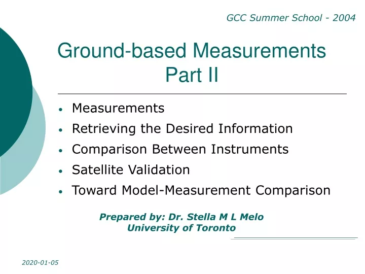
Ground-based MeasurementsPart II Measurements Retrieving the Desired Information Comparison Between Instruments Satellite Validation Toward Model-Measurement Comparison Prepared by: Dr. Stella M L Melo University of Toronto
AIRGLOW • What it is? • Proxy for MLT temperature, concentration and dynamics • How we measure? • Comparing T measurements using airglow with LIDAR T measurements.
AIRGLOW • What is it? • - “Spontaneous luminescence that rises from discrete transitions of the constituents of the atmosphere” (A. García-Muñoz, in preparation); • Has been used as proxy for atmospheric temperature, constituents and dynamics since back to the end of the 1950’s. • Main source: atomic oxygen photodissociated at higher altitudes.
AIRGLOW • O + O + M O2*+ M 250–1270 nm bands emission • O2* + O O(1S) + O2 557.7 nm emission • Not including ionosphere… • N + O NO* 180–280 nm emission • H + O3 OH*(v = 6-9) + O2 500–3000 nm bands emission (excess of energy 3.3 eV)
O2 O2 O2(b-x) 0-1 band measured by Keck I/HIRES (50 min integration) Slanger and Copeland, 2003
Airglow – Rocket measurements Rocket measurements – Alcantara (20S, 440W)
OH Dyer et al., 1997
Mars: Airglow Modeling – OH* By A. García Muños
Mars: Airglow Modeling – OH* Diurnal variation By A. García Muños
MLT Temperature from airglow • Atmospheric temperature is a basic parameter. • Mesopause (85-100 km) • Low temperature/low pressure • Transition from turbulent to molecular diffusion • Airglow can be used as proxy for MLT temperature • - OH vibrational bands • - well dispersed rotational lines • - extending from 400nm to 4mm • - intensity is relatively “easy” to measure Other planets!
AIRGLOW rotational temperature • Precision improve: • - as the signal to noise ratio improves (DR/R decreases • as the difference in rotational energy of the states (Fb-Fa) increases • -> two lines that are farther apart in the spectrum will give a more precise measurement of the temperature Issues about LTE…
Airglow imager Iwagami et al., JASTP, 2002
MLT Temperature from airglow • Airglow (nadir) observations do not contain direct altitude information • At the end of the 80’s - narrow-band sodium lidar begun to be used to remotely measure the altitude profile of the atmospheric temperature between 85-105 km • Data-set show: • bimodal character of the mesopause altitude • the occurrence of the Temperature Inversion Layer above 85 km • Lidar do not normally provide information about the horizontal structures
Lidar T profile • LIDAR – Light Detection and Range • Normally Lidar technique is used to measure Rayleigh scattering from which air density distribution is obtained. • By assuming hydrostatic and local thermodynamic equilibrium atmospheric temperature profiles can be calculated from the molecular backscatter profile. • Measurements are reliable form 30km up to 80 km altitude • Upper mesosphere: Na Lidar • Na fluorescence cross-section is 14 orders higher than the Rayleigh-scattering cross-section at 589 nm • Technique first proposed by Gibson et al., 1979 More on LIDAR? Carlo’s poster!
Lidar T profile • – Energy levels NaD2 lines • - Doppler-broadened fluorescence spectra of NaD2 transition. She et al., Applied Optics, 1992
Lidar T profile Melo et al., 2001
Compare Lidar and OH* Temperature • First proposed by von Zahn et al. (1987) - determine OH* altitude • OH* layer at 86 4 km • differences in temperature sometimes of up to 10 K • influence of: • clouds • differences in field of view • fast motions of the OH* layer due to gravity waves • assumed OH* layer shape
Lidar and OH* Temperature • She and Lowe (1998) compared temperature measured with lidar (Fort Collins) and from OH airglow (FTS): • Shape OH profile taken form WINDII measurements Generally, OH* rotational temperature can be used as a proxy of the atmospheric temperature at 87 ± 4 km
Observations at Fort Collins (41N, 105W) November 2-3, 1997 Nocturnal average: Lidar ~ 30 K > OH* At 4.38 UT: Lidar 65 K > OH*
Airglow Model • Photochemical model O3+H OH+O2 (3.3 eV) O + O2 + M O3 + M OH(n) + O H + O2 OH(n) + O2 OH(n-1) + O2 OH(n) + N2 OH(n-1) + N2 OH(n) OH(n-n) + hn (Based on Makhlouf et al. 1995)
OH* Rotational Temperature - Observations OH* response to a gravity wave based on Swenson and Gardner (1998) Lz~ 25 km
Recovering Mesospheric Atomic Oxygen Density Profile from Airglow Measurements Reed and Chandra (1975) parameterization Upper mesosphere-lower thermosphere [O]z = [O]max * EXP (0.5{1.0 + (Zmax - Z) / SH - EXP((Zmax - Z) / SH)}) Melo et al, 2001
3 [O] [O] [M] 2 Nightglow emissions - 80-110 km OI 5577 Green line O(1S 1D) O2 Atmospheric bands O2(b1Sg+ X3Sg-) OH Meinel bands OH(X3Pn’ X3Pn” ) O+O+M O2*+M O2*+O O(1S ) + O2 O2*+O2 O2+O2 O(1S )+O2 O +O2 O + O + M O2*+M O2* + O2 O2(b1Sg+)+O2 O2* + O O2 + O2 O2(b1Sg+ )+M Prod. H + O3 OH* + O2 OH* + M Prod. O + O2 + M O3 + M 2 [O] [M] [O] [M] 2 IOH IO2 [O] [M] IOI
Recovering Mesospheric Atomic Oxygen Density Profile from Airglow Measurements O-parameters recovered from the technique (solid line) compared to the input (dashed lines).
Recovering Mesospheric Atomic Oxygen Density Profile from Airglow Measurements Atomic oxygen density profiles (atoms/cm3) input (a) compared to retrieved (b) and the percentage difference (c).
TOH TO2
Hydroxyl Profile Measured by WINDII (symbols) and calculated (line) (13-06-93)
Airglow Imaging Systems for Gravity Wave Observations in the Martian Atmosphere • Stella M L Melo and K. Strong, University of Toronto • R. P. Lowe and P. S. Argall University of Western Ontario • A. Garcia Munoz, J. McConnell, I. C. McDade, York University • T. Slanger and D. Huestis, SRI International, California, USA • M. J. Taylor, Utah State University, USA • K. Gilbert, London, Canada • N. Rowlands, EMS Technologies Picture by Calvin J. Hamilton
Mars Airglow REmote Sounding - MARES MARES-Ground is a zenith-sky imaging system for ground-based observation of wave activity in the Martian atmosphere through measurement of the contrast in images of selected airglow features. MARES-GWIM is a satellite-borne nadir-viewing imager which will produce static images of wave-induced radiance fluctuations in two vertically separated night airglow layers in the atmosphere. - GWIM has been developed for Earth’s atmosphere - MARES-GWIM will be an adaptation of GWIM for the Martian atmosphere.