Download
1 / 87
880 likes | 1.09k Views
State Space Approach to Signal Extraction Problems in Seismology. Genshiro Kitagawa The Institute of Statistical Mathematics IMA, Minneapolis Nov. 15, 2001. Collaborators: Will Gersch (Univ. Hawaii) Tetsuo Takanami (Univ. Hokkaido) Norio Matsumoto (Geological Survey of Japan).

E N D
State Space Approach to Signal Extraction Problems in Seismology Genshiro Kitagawa The Institute of Statistical Mathematics IMA, Minneapolis Nov. 15, 2001 Collaborators: Will Gersch (Univ. Hawaii) Tetsuo Takanami (Univ. Hokkaido) Norio Matsumoto (Geological Survey of Japan)
Roles of Statistical Models Model as a “tool” for extracting information Data Information Modeling based on the characteristics of the object and the objective of the analysis. Unify information supplied by data and prior knowledge. Bayes models, state space models etc.
Outline • Method • Flexible Statistical Modeling • State Space Modeling • Applications • Extraction of Signal from Noisy Data • Automatic Data Cleaning • Detection of Coseismic Effect in Groundwater Level • Analysis of OBS (Ocean Bottom Seismograph) Data JASA(1996) + ISR(2001) + some new
Small Experimental, Survey Data Parametric Models + AIC Huge Observations, Complex Systems • Flexible Modeling • Smoothness priors • Automatic Procedures Change of Statistical Problems
Observation Unknown Parameter Noise Smoothness Prior Simple Smoothing Problem Infidelity to smoothness Infidelity to the data Penalized Least Squares Whittaker (1923), Shiller (1973), Akaike(1980), Kitagawa-Gersch(1996)
Automatic Parameter Determination via Bayesian Interpretation Crucial parameter Bayesian Interpretation Multiply by and exponentiate Smoothness Prior Determination of by ABIC (Akaike 1980)
Time Series Interpretationand State Space Modeling Equivalent Model State Space Model
Applications of State Space Model • Modeling Nonstationarity • in mean • Trend Estimation, Seasonal Adjustment • in variance • Time-Varying Variance Models, Volatility • in covariance • Time-Varying Coefficient Models, TVAR model • Signal Extraction, Decomposition
State Space Models Linear Gaussian Nonlinear Non-Gaussian Nonlinear Non-Gaussian Discrete state Discrete obs. General
Kalman Filter Initial Prediction Prediction Filter Filter Smoothing
Non-Gaussian Filter/Smoother Prediction Filter Smoother
True Normal approx. Piecewise Linear Step function Normal mixture Monte Carlo approx. Recursive Filter/Smootherfor State Estimation 0. Gaussian Approximation Kalman filter/smoother 1. Piecewise-linear or Step Approx.Non-Gaussian filter/smoother 2. Gaussian Mixture Approx. Gaussian-sum filter/smoother 3. Monte Carlo Based Method Sequential Monte Carlo filter/smoother
Sequential Monte Carlo Filter System Noise Predictive Distribution Importance Weight (Bayes factor) Filter Distribution Resampling Gordon et al. (1993), Kitagawa (1996) Doucet, de Freitas and Gordon (2001) “Sequential Monte Carlo Methods in Practice”
Self-Tuned State Space Model Time-varying parameter Augmented State Vector Non-Gaussian or Monte Carlo Smoother Simultaneous Estimation of State and Parameter
Tools for Time Series Modeling • Model Representaion • Generic: State Space Models • Specific: Smoothness Priors • Estimation • State: Sequential Filters • Parameter: MLE, Bayes, SOSS • Evaluation • AIC
Examples • Detection of Micro Earthquakes • Extraction of Coseismic Effects • Analysis of OBS (Ocean Bottom • Seismograph) Data
Observed Extraction of Signal From Noisy Data Component Models Basic Model
Extraction of Micro Earthquake 15 0 -15 15 0 -15 15 0 -15 4 2 0 -2 -4 -6 Observed Background Noise Seismic Signal Time-varying Variance (in log10) 0 400 800 1200 1600 2000 2400 2800
Extraction of Micro Earthquake Observed Earthquake Signal Background Noise
Extraction of Earthquake Signal Observed S-wave P-wave Background Noise
U-D N-S E-W P-wave 3D-Modeling S-wave P-wave U-D N-S E-W S-wave
Detection of Coseismic Effects Groundwater Level Precipitation Air Pressure Earth Tide dT = 2min., 20years Japan Tokai Area Observation Well Geological Survey of Japan 5M observations
Detection of Coseismic Effect in Groundwater Level Difficulties • Presence of many missing and outlyingobservations Outlier Missing • Strongly affected by barometric air pressure, earth tide and rain
Automatic Data Cleaning State Space Model Observation Noise Model
Mixture -5 -4 -3 -2 -1 0 1 2 3 4 5 -5 -4 -3 -2 -1 0 1 2 3 4 5 Model for Outliers
Missing and Outlying Observations Gaussian Mixture Original Cleaned
Detection of Coseismic Effects 1981 1982 1983 1984 1985 1986 1987 1988 1989 1990 Strongly affected the covariates such as barometric air pressure, earth tide and rain Difficult to find out Coseismic Effect
Pressure Effect Air Pressure Pressure Effect
Extraction of Coseismic Effect Component Models Observation Trend Air Pressure Effect Earth Tide Effect Observation Noise
Precipitation Effect Pressure, Earth-Tide removed Original
Extraction of Coseismic Effect Component Models Observation Trend Air Pressure Effect Earth Tide Effect Precipitation Effect Observation Noise
Air Pressure Effect Earth Tide Effect Precipitation Effect Extraction of Coseismic Effects Groundwater Level M=4.8, D=48km min AIC model m=25, l=2, k=5 Corrected Water Level
M=4.8 D=48km M=6.0 D=113km M=6.8 D=128km M=7.7 D=622km M=7.9 D=742km M=5.7 D=66km M=6.2 D=150km M=5.0 D=57km M=7.0 D=375km Detected Coseismic Effect Original T+P+ET T+P+ET+R Signal
Original Air Pressure Effect Earth Tide Effect P & ET Removed Precipitation Effect P, ET & R Removed Min AIC model m=25, l=2, k=5
1981 1982 1981 1982 M=7.0 D=375km M=4.8 D=48km 1983 1984 M=6.0 D=113km M=6.8 D=128km 1983 1984 M=7.7 D=622km M=7.9 D=742km M=5.7 D=66km M=6.2 D=150km M=5.0 D=57km 1985 1986 1985 1986 M=6.0 D=126km 1987 1988 1987 1988 M=6.7 D=226km 1989 1990 1989 1990 M=5.7 D=122km M=6.5 D=96km Coseismic Effect
> 16cm > 4cm >1cm Rain Water level Magnitude Distance Coseismic Effect Earthquake Water level Effect of Earthquake
Findings • Drop of level Detected for earthquakes with • M > 2.62 log D + 0.2 • Amount of drop ~ f( M- 2.62 log D ) • Without coseismic effect water level increases • 6cm/year • increase of stress in this area?
Sea Surface OBS Exploring Underground Structure by OBS(Ocean Bottom Seismogram) Data Bottom
4 Channel Time Series N=15360, 98239 series Observations by an Experiment • Off Norway(Depth 1500-2000m) • 39 OBS, (Distance: about 10km) • Air-gun Signal from a Ship (982 times: Interval 70sec., 200m) • Observation(dT=1/256sec., T =60sec., 4-Ch) Hokkaido University + University of Bergen
An Example of the Observations OBS-4 N=7500 M=1560 OBS-31 N=15360 M=982 Low S/N High S/N
Direct wave, Reflection, Refraction Refraction Wave Direct Wave Reflection Wave
Objectives Estimation of Underground Structure Intermediate objectives Detection of Reflection & Refraction Waves Estimation of parameters (hj , vj)
Time series at hypocenter (D=0) Wave(011) Wave(00011) Wave(0) Wave(000) Wave(00000)
Model for Decomposition Self-Organizing Model
Decomposition of Ch-701 (D=4km) Observed