Download
1 / 60
1.68k likes | 3.51k Views
Fuzzification. By considering quantities as uncertain: Imprecision Ambiguity Vagueness Membership Assignment Many ways to do it!. Intuition. Using our intelligence and understanding.

E N D
Fuzzification By considering quantities as uncertain: Imprecision Ambiguity Vagueness Membership Assignment Many ways to do it!
Intuition Using our intelligence and understanding. Intuition involves contextual and semantic knowledge about an issue. It can also involve linguistic truth-values about the knowledge. Note: they are overlapping.
Inference Using knowledge to perform deductive reasoning. Example: Let U be a universe of triangles. U = { (A B C) | A > B > C > 0 A + B + C = 180° } We can define the following 5 types of triangles: I: Approximate isosceles triangle R: Approximate right triangle IR: Approximate isosceles and right triangle E: Approximate equilateral triangle T: Other triangles
Inference µI(A B C) = 1 – 1/60° min(A – B,B – C) µR(A B C) = 1 – 1/90° |A - 90°| IR = I R µIR(A B C) = min [ µI(A B C), µR(A B C) ] = 1 – max[1/60 min(A – B,B – C),1/90 |A - 90|] E(A B C) = 1 – 1/180 (A – C) T = (I R E)’ = I’ R’ E’ = min{1 - µI,1 -1 µR,1 - µE} = 1/180 min{3(A – B),3(B – C),2| A - 90|,A – C}
Rank Ordering Assessing preference by a single individual, a pole, a committee, and other opinion methods can be used to assign membership values to a fuzzy variable. Preference is determined by pair wise comparisons which determine the order of memberships.
Angular Fuzzy Sets Angular Fuzzy sets are defined on a universe of angles with 2 as cycle. The linguistic values vary with and their memberships are t() = t tan() Angular Fuzzy sets are useful for situations: Having a natural basis in polar coordinates, or the variable is cyclic.
Training Testing R1 R2 R3 Neural Networks We have the data sets for inputs and outputs, the relationship between I/O may be highly nonlinear or not known. We can classify them into different fuzzy classes. Then, the output may not only be 0 or 1!
Neural Networks memberships Once the neural network is trained and tested, it can be used to find the membership of any other data points in the fuzzy classes (# of outputs)
Genetic Algorithms Crossover Mutation random selection Reproduction Chromosomes Fitness Function Stop (terminate conditions) Converge Reach the #limit
Inductive Reasoning Deriving a general consensus from the particular (from specific to generic) The induction is performed by the entropy minimization principle, which clusters most optimally the parameters corresponding to the output classes. The method can be useful for complete systems where the data are abundant and static. The intent of induction is to discover a law having objective validity and universal application.
Inductive Reasoning Particular General Maximize entropy Computing mean probability Minimize entropy The entropy is the expected value of information. Many entropy definitions! A survey paper
Inductive Reasoning One example: S(x) = p(x) Sp(x) + q(x) Sq(x) Sp(x) = -[P1(x) ln(P1(x)) + P2(x) ln(P2(x))] Sq(x) = -[q1(x) ln(q1(x)) + q2(x) ln(q2(x))]
Inductive Reasoning Where: nk(x): # of class k samples in [x1,x1+x] n(x): Total # of samples in [x1,x1+x] Nk(x): # of class k samples in [x1+x,x2] N(x): Total # of classes in [x1+x,x2] n = Total # of samples in [x1,x2] Move x in [x1,x2], and compute the entropy for each x to find the maximum / minimum entropy. Note: there are many approaches to compute entropy.
● Defuzzification (Fuzzy-To-Crisp conversions) Using fuzzy to reason, to model Using crisp to act Like analog digital analog Defuzzification is the process: round it off to the nearest vertex. Fuzzy set (collection of membership values).
Defuzzification (Fuzzy-To-Crisp conversions) A vector of values reduce to a single scalar quantity: most typical or representative value. Fuzzification – Analysis – Defuzzification – Action -cuts for fuzzy sets (-cuts, some books) A, 0 < <1 A = {x | A(x) > } Note: A is a crisp set derived from the original fuzzy set. [0,1] can have an infinite number of values. Therefore, there can be infinite number of -cut sets.
Defuzzification (Fuzzy-To-Crisp conversions) Example: A = {1/a + 0.9/b + 0.6/c + 0.3/d + 0.01/e + 0/f} A1 = {a} or A1 == {1/a + 0/b + 0/c + 0/d + 0/e + 0/f} A0.9 = {a,b} A0.3 = {a,b,c,d} A0.6 = {a,b,c} A0.01 = {a,b,c,d,e} A0 = x = {a,b,c,d,e,f}
Defuzzification (Fuzzy-To-Crisp conversions) • -cut re-scales the memberships to 1 or 0 • The properties of -cut: • (A B) = A B • 2. (A B) = A B • 3. (A’) (A)’ except for x = 0.5 • 4. A A < and 0 < < 1 • A0 = X • Core = A1 • Support = A0+ • Boundaries = [A0 + A1]
0.6 0.3 R = Defuzzification (Fuzzy-To-Crisp conversions) -cuts for fuzzy relations
R1 = R0.9 = Defuzzification (Fuzzy-To-Crisp conversions) We can define -cut for relations similar to the one for sets R = {(x y) | R(x y) > } R0 = E
Defuzzification (Fuzzy-To-Crisp conversions) -cuts on relations have the following properties: (R S) = R S (R S) = R S (R’) (R)’ R< R and 0 1
Defuzzification Methods fuzzy set a single scalar quantity fuzzy quantity precise quantity O1 O2 O = O1 O2
Defuzzification Methods A fuzzy output can have many output parts Many methods can be used for defuzzification. They are listed in the following slides
1 1 z* z z* z Defuzzification Methods Max-membership principle c(Z*) c(z) z Z Centroid principle Note: It relates to moments.
.9 .5 0 a b z 1 0 a z* b z Defuzzification Methods Weighted average method (Only valid for symmetrical output membership functions) Mean-max membership (middle-of-maxima method)
Defuzzification Methods Example: A railroad company intends to lay a new rail line in a particular part of a county. The whole area through which the new line is passing must be purchased for right-of-way considerations. It is surveyed in three stretches, and the data are collected for analysis. The surveyed data for the road are given by the sets , where the sets are defined on the universe of right-of-way widths, in meters. For the railroad to purchase the land, it must have an assessment of the amount of land to be bought. The three surveys on the right-of-way width are ambiguous , however, because some of the land along the proposed railway route is already public domain and will not need to be purchased. Additionally, the original surveys are so old (circa 1860) that some ambiguity exists on the boundaries and public right-of-way for old utility lines and old roads. The three fuzzy sets , shown in the figures below, represent the uncertainty in each survey as to the membership of the right-of-way width, in meters, in privately owned land. We now want to aggregate these three survey results to find the single most nearly representative right-of-way width (z) to allow the railroad to make its initial estimate
Defuzzification Methods Centroid method:
Defuzzification Methods Weighted-Average Method: Mean-Max Method:
Defuzzification Methods According to the centroid method,
Defuzzification Methods The centroid value obtained, z*, is shown in the figure below:
Defuzzification Methods According to the weighted average method:
Defuzzification Methods Center of sums Method Faster than any defuzzification method Involves algebraic sum of individual output fuzzy sets, instead of their union Drawback: intersecting areas are added twice. It is similar to the weighted average method, but the weights are the areas, instead of individual membership values.
Defuzzification Methods z1 = 4 z2 = 8 or
Defuzzification Methods Center of Sums Method
Defuzzification Methods Using Center of sums: S1 = 0.5 * 0.5(8+4) = 3 S2 = 0.5 * 1 * 4 = 2 Center of the largest area: if output has at least two convex sub-regions Where Cm is the convex sub-region that has the largest area making up Ck. (see figure)
Defuzzification Methods Center of sums method
Defuzzification Methods First (or Last) of Maxima method This method uses the overall output or union of all individual output fuzzy sets to determine the smallest value of the domain with maximized membership degree in each output set. The equations for z* are as follows: First, the largest height in the union is determined: Then the first of the maxima is found:
Defuzzification Methods First (or last) of Maxima method An alternative to this method is called the last of maxima, and it is given by: Supremum (Sup): the least upper bound Infimum (Inf): the greatest lower bound
Defuzzification Methods Continuation of the railroad example, the results of the different methods can be shown graphically as follows:
x y f(x) Fuzzy Arithmetic, Numbers, Vectors The Extension Principle How to find y if x is fuzzy, f is fuzzy or both are fuzzy
Crisp function, Mapping and Relation For a set A defined on universe X, its image, set B on the universe Y is found from the mapping B = f(A) = { y | x A, y = f(x) B is defined by its characteristic value XB(y) = Xf(A)(y) = XA(x) Note: means max y = f(x)
Crisp function, Mapping and Relation Example: A = {0/-2 +0/-1 +1/0 +1/1 +0/2} X = {-2,-1,0,0,1,2} If y = |4x| + 2 Y = {2,6,10} XB(2) = {XA(0)} = 1 XB(6) = {XA(-1),XA(1)} = {0,1} = 1 XB(10) = {XA(-2),XA(2)} = {0,0} = 0 B = {1/2 + 1/6 + 0/10} or B = {2,6}
R = Crisp function, Mapping and Relation We may consider the universe X = {-2,-1,0,1,2} and universe Y = {0,1,2,…,9,10} The relation describing this mapping
Crisp function, Mapping and Relation If A = {0/-2 + 0/-1 + 1/0 + 1/1 + 0/2} Then, B = A R XB(y) = (XA(A) XR(x y)) 1 for y = 2,6 = 0 otherwise or B = {0/0 + 0/1 + 1/2 + 0/3 + 0/4 + 0/5 + 1/6 + 0/7 + 0/8 + 0/9 + 0/10} x X
Function of Fuzzy Sets – Extension Principle B = f(A) If A is fuzzy, B is also fuzzy. µB(y) = µA(x) Fuzzy Vectors: f(x) = y
Function of Fuzzy Sets – Extension Principle General case Let A1,A2,…An be defined on X1,X2,…,Xn Then B = f(A1,A2,…,An) This is called Zadeh’s extension principle.