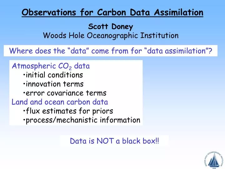
Observations for Carbon Data Assimilation

1. Observations for Carbon Data Assimilation Scott Doney Woods Hole Oceanographic Institution Where does the “data” come from for “data assimilation”? • Atmospheric CO2 data • initial conditions • innovation terms • error covariance terms • Land and ocean carbon data • flux estimates for priors • process/mechanistic information Data is NOT a black box!!

2. Atmospheric Inverse Modeling of CO2 Concentration (observed samples) Sources & Sinks (solved for) Transport (modeled) + =

3. How data enters the problem (1) Variational Assimilation Adjust model state “x” (atmospheric CO2 field) to minimize cost function J: Deviation of x from “background” Deviation of x from “observations” • So where do we get: • y0(t) data for innovation (model-data misfit) • R data error covariance • B model error covariance

4. Some Issues to Ponder • Atmosphere CO2 drastically under-sampled • original design for marine background air • mostly discrete surface samples • NWP deg. freedom O(107); 6 hourly observations O(104-105) • CO2 weekly observations O(102-103) • Small signal on large background variability • surface North-south difference ~2.5 ppmv • zonal continent to land contrast <1 ppmv • measurement precision • accuracy in time & across stations and networks • reduce systematic biases!!

5. Some Issues to Ponder • Representativeness of data y0 • “footprint” of observation • & mismatch with model grid • local heterogenity or point sources • aliasing of unresolved frequencies/wavenumbers (e.g., diurnal cycle) • data selection (i.e., exclude “unrepresentative” • observations)

6. CCSM Climate Working Group Board of Trustees Reception National Science Board Breakfast ASP Reviews CO2 Concentration in the Outer Damon Room, NCAR Mesa Lab, 2/7 – 2/9/06

7. Multiple Time/Space Scales

8. In-situ Atmospheric Observing Network Discrete surface flasks (~weekly) Continuous surface (hourly) observatories Tall towers continuous (hourly) Aircraft profiles (~weekly)

9. Surface Observatory

10. Seasonal CO2: Continental vs Oceanic Sites • CO2 seasonal cycle attenuate, but still coherent, far away from source/sink region • Peak-trough amplitude of seasonal cycle ~ 30 ppmv (~10%)

11. 10 ppmv Weather Cycles: CO2 is variable Modeled: one day in July [LSCOP, 2002] TURC/NDVI Biosphere; Takahashi Ocean ; EDGAR Fossil Fuel [U. Karstens and M. Heimann, 2001] On DT~5 days, Dx ~ 1000 km CO2 variability in the boundary layer ~ 10 ppmv (3 %)

12. Diurnal CO2: Highly variable in boundary layer Calm night: stably stratified boundary layer Well-mixed PBL • Diurnal cycle of photosynthesis and respiration •  > 60 ppmv (20%) diurnal cycle near surface • Varying heights of the planetary boundary layer (varying mixing volumes)

14. Vertical Profiles (free troposphere) 384 372 2006 2005 DATE

15. Aircraft Campaigns COBRA 2000

16. Surface Fluxes => Atmospheric CO2

17. Orbiting Carbon Observatory(Planned Fall 2008 launch) • Estimated accuracy for single column ~1.6 ppmv • 1 x 1.5 km IFOV • 10 pixel wide swath • 105 minute polar orbit • 26º spacing in longitude between swaths • 16-day return time

18. How data enters the problem (2) Separating transport, initial conditions & surface fluxes Analysis at time i => forecast at time i+1 transport fluxes 4D Variational methods: adjust initial conditions to better match future data initial conditions Deviation of x from “observations” Deviation of initial conditions from “prior” Deviation of fluxes from “prior”

19. NEE = GPP – Reco NEE is measured at the tower GPP Photosynthesis (Daytime only) Ecosystem Respiration typically based on nighttime NEE & air temperature & ? Reco = Rhetero + Rauto CO2 CO2 CO2 Adapted from Gilmanov et al.

20. Eddy-Flux Towers Vertical velocity (mean and anomaly) CO2 concentration (mean and anomaly) Vertical CO2 flux

21. FluxNet Tower Sites

22. Diurnal and Seasonal Cycle

23. Time-scale character of carbon fluxes Variability is at a maximum on the strongly forced time scales They have an annual sum of ~0 Modeling the carbon storage time scales is much more difficult Diurnal Seasonal

25. Tall-TowerFootprint 6 4 2 South-North Direction (km) 0 -2 -4 -6 -6 -4 -2 0 2 4 6 West-East Direction (km) Shrubland Barren Forested Wetland Lowland Shrub Wetland Mixed Dec/Con Mixed BL Deciduous Aspen Mixed Coniferous Pine Grassland Water Urban/Dev/Ag (Wang, 2005)

26. Forest Inventory Analysis: Slow Process Observations • Plot-scale measurement of carbon storage, age structure, growth rates: 170,000 plots in US! • Allows assessment of decadal trends in carbon storage

27. Air-Sea CO2 Flux Estimates Takahashi F = k s(pCO2air - pCO2water) = ksDpCO2 Kinetics transfer velocity Thermodynamics -undersampling & aliasing of surface water pCO2 -transfer velocity k empirically derived from wind speed relationships

29. Gas Transfer Velocity

31. Generating a Global Flux Map

32. In-Situ Sensors and Autonomous Platforms Moorings/drifters (DpCO2, pH, DIC, NO3) Chavez et al. Profiling ARGO floats (also AUVs, caballed observatories) Riser et al.

33. JGOFS/WOCE global survey (1980s and 1990s) -Global baseline (hydrography, transient tracers, nutrients, carbonate system) -Improved analytical techniques for inorganic carbon and alkalinity (±1-3 mmol/kg or 0.05 to 0.15%) -Certified Reference Materials -Data management, quality control, & public data access

35. Ocean Inversion Method -Ocean is divided into n regions (n = 30, aggregated to 23) -Basis functions for ocean transport created by injecting dye tracer at surface in numerical models

36. Simple Inversion Technique • Basis functions are model simulated footprints of unit emissions from a number of fixed regions • Estimate linear combination of basis functions that fits observations in a least squares sense. • Inversion is analogous to linear regression footprints fluxes obs Premultiply both sides by inverse of A estimated fluxes