Download
1 / 48
480 likes | 663 Views
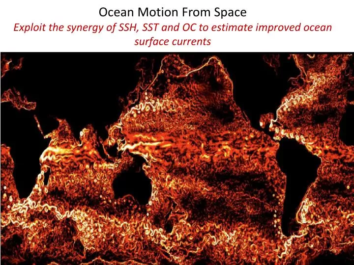
Ocean Motion From Space Exploit the synergy of SSH, SST and OC to estimate improved ocean surface currents. Ocean Motion From Space Exploit the synergy of SSH, SST and OC to estimate improved ocean surface currents. The needs

E N D
Ocean Motion FromSpace Exploit the synergy of SSH, SST and OC to estimateimprovedocean surface currents
Ocean Motion FromSpace Exploit the synergy of SSH, SST and OC to estimateimprovedocean surface currents • The needs • Measuringoceancurrentsfromspace: existingapproaches • Limits of the altimeter system • Improvingaltimetercurrentsthrough the mergingwith OC/SST data • The Mercatini et al, 2010 approach • The challenges • Workplan
Ocean Motion FromSpace The needs Search And Rescue navigation Iceforecasting fisheries aquaculture Climate change research Shiprouting coastal development and management Offshore operations Maritime Pollution
The GlobCurrent Project • The GlobCurrent Project was kicked-off in October 2013. The project has a 3-years duration and is supported by the European Space Agency (ESA) under the Data User Element (DUE) programme. • The overall objective of the project is to advance the quantitative estimation of ocean surface currents from satellite sensor synergy and demonstrate impact in user-led scientific, operational and commercial applications that, in turn, will increase the uptake of satellite measurements. • The project is led by NERSC with expertise from four partners, i.e. IFREMER, CLS, PML, ISARDSAT
Measuringoceancurrentsfromspace: existingapproaches • At the moment there is no satellite observing system that provides direct observations of the ocean surface currents. • However, a large variety of active and passive remote-sensing instruments have been put into orbit in the last few decades providing continuous, global information about the ocean. • This includes altimeters, scatterometers, Synthetic Aperture Radars (SAR), imaging radiometers operating at different wavelengths, spectrometers. • Estimates of the surface current can be retrieved by transformation of these satellite-measured quantities based on a range of assumptions, feature tracking methods and empirical based retrieval algorithms.
Measuringoceancurrentsfromspace: existingapproaches Altimetry, by providing global, accurate and repetitive measurements of the Sea Surface Height (SSH), has been by far the most exploited system for the study of the ocean surface currents variability over the last 20 years
= G + h Measuredwithaltimetryat cm accuracy Signal of interest for oceanographers hO hA Geoid: poorlyknownat short scales =hO-hA Altimeter missions repetitivity = G + G The altimeterPrinciple orbit h Geoid AltimeterSeaLevel Anomalies h’P Example of SeaLevelAnomalyaftermultimissionmapping E
= G + h Measuredwithaltimetryat cm accuracy Signal of interest for oceanographers Geoid: poorlyknownat short scales Altimeter missions repetitivity = G + SSALTO DUACS: ’computed relative to a 7 yearsmean profile (P=1993-1999) In order to reconstruct the dynamictopography h from the SeaLevelAnomalyh’= ’the missing component is: The oceanMeanDynamicTopography (MDT) for the period 1993-1999 The altimeterPrinciple AbsoluteDynamicTopographyh = AltimeterSeaLevel Anomalies h’93-99 + MeanDynamicTopography
Calculating the oceanMeanDynamicTopography: The direct method <h>P(x,y)=< η >P(x,y)–G(x,y) η(t,x,y) = G(t,x,y) + h(t,x,y) MDT=MSS–GEOID MSS 9399 GEOID m
Calculating the oceanMeanDynamicTopography: The direct method <h>P(x,y)=< η >P(x,y)–G(x,y) η(t,x,y) = G(t,x,y) + h(t,x,y) MDT9399=MSS9399–GEOID cm
Rc=400 km Rc=200 km Calculating the oceanMeanDynamicTopography: The direct method MDT9399 Gaussianfilter cm Rc=300 km
Calculating the oceanMeanDynamicTopography: The direct method 20 years of MSS improvements MSS OSU 95 MSS CLS_SHOM98 MSS CLS01 MSS DNSC08 MSS DTU10 MSS CNES_CLS_2011
Calculating the oceanMeanDynamicTopography: The direct method 20 years of GEOID improvements Satellite-only geoid models RMS differences (in cm) between geoid models and GOCE-TIM-R3 filtered at 100km (on oceans) 120 98 50 44 5 1995 1999 2003 2005 2010
20 YEARS OF Geoid IMPROVEMENTS: Impact on MDT determination 1995
20 YEARS OF Geoid IMPROVEMENTS: Impact on MDT determination 1999
20 YEARS OF Geoid IMPROVEMENTS: Impact on MDT determination 2003
20 YEARS OF Geoid IMPROVEMENTS: Impact on MDT determination 2005
20 YEARS OF Geoid IMPROVEMENTS: Impact on MDT determination 2006
20 YEARS OF Geoid IMPROVEMENTS: Impact on MDT determination 2009
20 YEARS OF Geoid IMPROVEMENTS: Impact on MDT determination GRACE: Resolution 150 km 2010
20 YEARS OF Geoid IMPROVEMENTS: Impact on MDT determination GRACE: Resolution 125 km 2010
20 YEARS OF Geoid IMPROVEMENTS: Impact on MDT determination GOCE: Resolution 125 km 2012
Example in the GulfstreamRegion MeanGeostrophicVelocities 2009: 5 years of GRACE data In-Situ mean velocities MSS CLS01-EIGEN - GRGS.RL02 300 km
Example in the GulfstreamRegion MeanGeostrophicVelocities 2009: 5 years of GRACE data In-Situ mean velocities SMO CLS01-EIGEN-GRGS 133 km
Example in the GulfstreamRegion MeanGeostrophicVelocities 2011: 1 year of GOCE data In-Situ mean velocities MSS CLS10 - EGM-DIR-V3 100 km
Computingthe oceanMeangeostrophicvelocitiesfrom in-situ and altimeter data (=syntheticmeanvelocities) SVP- Drifting buoy velocities 1993-2010 (u,v) (u’a,v’a) cm/s Ateach position r and time t for which an oceanographic in-situ measurement of surface velocityu(r,t),v(r,t)isavailable - the altimeter velocity anomaly u’a(r,t),v’a(r,t) is interpolated to the position/date of the in-situ data. - the in-situ data isprocessed to match the physical content of the altimetermeasurement (geostrophiccurrents) - the altimetervelocityanomalyissubtractedfrom the in-situ velocity
Meangeostrophiccurrentsfrom the MDT CNES-CLS13 (Rio et al, in preparation)
Altimetry Topex-Poseidon/Jason ERS/Envisat Impact the spatial and temporal resolutioncapability Impact the spatial coveragecapability: Spatial coveragelimited to 66°N/S for TP/Jason , 82°N/S for ERS/Envisat Multi-mission merging to obtaingriddedmaps of altimeter data. Final resolution of gridded products depends on the number of satellites flyingat the same moment and theirorbitcharacteristics Maps of surface velocitiesusing the geostrophic approximation:
Altimeter Constellation history Spatial resolutionachieved for a 10 days temporal resolution 2 satellites 250-300km 4 satellites 100 km 3 satellites 150 km
Altimetry Limitation • Spatio temporal resolutionachievable Time-space diagram depicting the characteristic temporal and spatial scales of the dominant surface current features in the ocean. Adapted from Chelton, (2001). The dashed lines indicate the approximate lower bounds of the space and tie scales that can be resolved in SSH fields constructed from multimission altimeter measurements (3 satellite configuration) • Physical content of the currents: only the geostrophic component isobtained • Errorincreasestoward the coast and athigh latitudes (seasonalicecoverage, limited satellite coverage)
Measuringoceancurrentsfromspace: Use of tracer information
MCC methodology From http://ccar.colorado.edu/colors/mcc.html
MCC methodology From http://ccar.colorado.edu/colors/mcc.html The MCC method (Emery et al, 1986) is an automated procedure that calculates the displacement of small regions of patterns from one image to another. The location of the subwindow in the second image that produces the highest cross-correlation with the subwindow in the first image indicates the most likely displacement of that feature. The velocity vector is then calculated by dividing the displacement vector by the time separation between the two images. The solid boxes in the first image is the pattern to search for in the second image. The dashed boxes in the second image is the “search window".
MCC methodology From http://ccar.colorado.edu/colors/mcc.html Limitations • Cloud-cover and isothermal/isochromatic ocean surface conditions drastically limit the spatial and temporal velocity coverage provided by the MCC method. Clouds block the ocean surface in both thermal and ocean color imagery, and there are no features for the MCC method to track in isothermal/isochromatic regions. • Accurate spatial alignment and coregistration of the imagery used in feature tracking is required. Consequently, the technique has been more often used in coastal regions, where landmarks are available to renavigate the satellite data. • MCC techniques work well for intervals between images of 6-24 hrs, but are not so reliable for longer gaps due to evolution of the features, including rotation and shear.
E-SQG Method • General concept: Exploit the correlationbetweenSST and SSH(Jones et al. 1998) : - Positive (0.2-0.6) at large scale (>1000km) - Strong(0.7) at short scales in strong gradients areas SSH 1/3° (SSALTO/DUACS) SST 1/4° (AMSR-E V5) • Key point of SQG theory: in the horizontal Fourier transform domain SST anomaly Streamfunction Surface Density Anomalies Currents N(z)=Neffthe effective Brunt-Vaisalafrequency (constant stratification assumed)
E-SQG Method Courants issus de SSH Courants issus de SST • Limitations • The SQG methodisvalid in baroclinicinstabilities areas, and strong gradients areas (ACC, Gulfstream, Kuroshio…) • In addition, the validity of the SQG approximation islimited to cases when the SST is a good proxy of the densityanomalyat the base of the mixed layer, whicheffectivelyhappensafter a mixed-layer deepeningperiod. Therefore the ideal situation for the application of thismethodwouldbeafterstrongwindevents. • Limited to the retrieval of mesoscale (30-300km), not the large scalecurrents • Isern-Fontanet et al, 2006, 2008: the reconstruction can be still improved if we exploit the synergy between SST and SSH:
On the use of submesoscale information for the control of ocean circulations, Gaultier L., Verron J., Brankart J.M., Titaud O. and Brasseur P. Journal of Marine Systems, 2013 FSLE (in day−1) derived from the geostrophic AVISO velocity first week of July, 2004 Background velocity to be corrected: map of velocity derived from AVISO altimetric observations at 1/8 resolution: Tracer used as a dynamic informa- tion: high resolution SST images from MODIS sensor at 1 km resolution: Finite-Size LyapunovExponents (FSLE) measure stirring in a fluid, It is a connection between sub-mesoscale dynamics and tracer stirring. FSLE is the exponential rate at which two particles separate from a distance δ0 to δf : Geostrophic Velocity (in m.s−1) over the SSH (in cm) on the first week of July, 2004 from AVISO. SST image from MODIS sensor (in C) on July 2nd, 2004 Method: Modify the altimeter velocity field so as to minimize the cost function J that measures the distance between the binarized normalized gradient of SST and the binarized FSLE (u) (as a proxy of the velocity u).
Ocean Motion FromSpace Exploit the synergy of SSH, SST and OC to estimateimprovedocean surface currents SSH OC SST
Ocean Motion FromSpace Exploit the synergy of SSH, SST and OC to estimateimprovedocean surface currents Starting point: Inverse methods (Kelly et al, 1989): Require the velocity field to obey the tracer evolution equation and inverse it for the velocity vector: c(x, y, t) is thenormalizedconcentration of a tracer known from successive satellite observations u,vis the velocityfield f(x,y,t) represents the source and sinkterms Challenge: there is no contribution to tracer advection from the along-track gradient velocity, or from either components in regions of negligible gradients. -> only cross-gradient velocity information can be retrieved from the tracer distribution at subsequent times in strong gradients areas.
Ocean Motion FromSpace Exploit the synergy of SSH, SST and OC to estimateimprovedocean surface currents Solution from Mercatini et al, 2010 : Use a background velocity information (ubck, vbck) so that the satellite tracer information is used to obtain an optimized ‘blended’ velocity (uopt, vopt). The authors tested the implementation of the method for the specific application of oil spill monitoring using background velocities from a numerical model.
Ocean Motion FromSpace Exploit the synergy of SSH, SST and OC to estimateimprovedocean surface currents Our Approach Apply the methodology on successive OceanColor and SST images using the lowresolution, geostrophicaltimetervelocities as background velocities. -> Altimetervelocitieswillbeimproved in term of resolution by the higherresolution information contained in the SST/OC images -> Altimetervelocitieswillbeimproved in term of physical content (ageostrophicterms) by the total velocity information derivedfrom the SST/OC images -> The application of the method on both OC and SST images increase the overall spatial and temporal velocity coverage. In addition, ocean colour can also resolve isothermal flow, i.e. in regions where the different water masses do not have distinctive temperatures.
Ocean Motion FromSpace Exploit the synergy of SSH, SST and OC to estimateimprovedocean surface currents • Two main issues: • Need for high spatial and temporal resolution time series of cloud free images. • Visible/infrared spectral band radiometers: very high spatial resolution (0.3-1km, 4km in the case of geostationary satellites) but their availabilities are severely limited by the presence of clouds. Microwave imagers provide accurate satellite SST measurements under clouds but the spatial resolution is much lower (about 50 km). • -> merging techniques to compute cloud-free images of SST and Ocean colour from the different available datasets. The drawback of these merged products is that adjacent pixels may have been actually measured at different times and from different sensors. The impact on the accuracy of the derived velocities will need to be carefully assessed. • Accurate prescription of the “Source” and “Sink” terms of the evolution equation is needed in cases where the tracer evolution is not driven only by advection. • SST • Insolation • net infrared radiation • sensible and latent heat fluxes. • -> These terms may be measured directly or indirectly via a Bulk Formulae. • OC • The main contributor to OC is phytoplankton, which is both a passive tracer transported by water circulation and an active biomass growing under favorable conditions (light, nutrients, etc.)
Ocean Motion FromSpace Exploit the synergy of SSH, SST and OC to estimateimprovedocean surface currents The applicability of the method will be tested using an OSSE (Observing System Simulation Experiment) based on ocean numerical modeling outputs Model outputs Nominal conf SSTm Ocm Um,Vm Degraded Model outputs SSTtest OCtest Altimeter data Ubck, Vbck MER10 BlendedVelocities Uopt, Vopt • SSTtest, OCtest: Test a number of configurations regarding the SST and OC observing systems: • different time acquisition of adjacent pixels in high resolution SST and OC merged products • different parameterizations for the “source” and “sink” terms of the tracer evolution equation • impact of growing time steps between two consecutive images
Ocean Motion FromSpace Exploit the synergy of SSH, SST and OC to estimateimprovedocean surface currents Task description Task 1 Gaining expertise on Sea Surface Temperature and Ocean color measurements from space Task 1.1: Bibliographical work Task 1.2: Intercomparison of merged images and Level 3 single sensor images in term of spatial/temporal resolution Task1.3: Analysis of the different driving mechanisms of the SST and Ocean color evolution, and their relative contribution (advection versus diffusion versus ) Task 1.4: Selection of areas/periods with successive cloud free high resolution images • Task 2 Observation System Simulating Experiments • Task 2.1: Use of model fields to create synthetic maps of Sea Surface Temperature/Ocean color • Task 2.2: Implement the MER10 methodology to create blended velocities from altimetry and synthetic SST/Ocean color images • Task 2.3: Sensitivity studies
Ocean Motion FromSpace Exploit the synergy of SSH, SST and OC to estimateimprovedocean surface currents Task description Task 3: Implementation and testing of the method on real datasets Task3.1: Testing the method capacity of retrieving shortest scales of the geostrophic currents we will consider a study period for which four altimeters have been flying simultaneously (2002-2008) and for which therefore altimeter sea level maps (and the corresponding geostrophic velocities) have been computed using the four altimeter data measurements. Concurrent maps computed using only 2 altimeters out of the four available will be used as background velocities (with therefore a decreased spatial resolution) and the methodology will be applied using high resolution SST and OC maps. We will check that the resulting “blended” surface velocities compare better to the full resolution, four altimeter data based geostrophic velocities than the background velocities. Task3.2: Testing the method capacity of retrieving the ageostrophic component of the currents We will apply the methodology using the altimeter surface velocities as background for a given study period and compare the resulting “blended” velocities to the total velocities provided by the OSCAR (Bonjean et al, 2002) or SURCOUF (Larnicol et al, 2005) products that also include the Ekman current component.
Ocean Motion FromSpace Exploit the synergy of SSH, SST and OC to estimateimprovedocean surface currents Task description Task 4: Organization of the “OceanMotionFromSpace” workshop Task 5: Validation Task 5.1: Intercomparison to MCC methodology Task 5.2: Intercomparison to SQG methodology Task 5.3: Intercomparison synthesis Task 6: Outreach activity Task 7: Scientific paper writting
Ocean Motion FromSpace Exploit the synergy of SSH, SST and OC to estimateimprovedocean surface currents 9 months Gantt Diagram 1/3/2014 1/3/2015 Task 1 1/4/2014 1/10/2014 Task 2 1/9/2014 1/3/2015 Task 3 1/1/2015 31/8/2015 Task 4 1/1/2015 15/3/2015 Task 5 1/3/2014 31/8/2015 Task 6 OceanMotionFromSpace Workshop 15/3/2015 Project Presentation Seminar Soul Food Festival 15/5/2015 15/3/2014 2014 2015 2014 mars mai juil. sept. nov. janv. mars mai juil. 2015 1/3/2014 31/8/2015 Beginning of project End of project