Download
1 / 33
370 likes | 904 Views
BEIT, 6th Semester. Books:. Getting Started with MATLAB"- Rudra PratapDigital Signal Processing "- Sanjit K. Mitra.Digital Signal Processing-A Practitioner's Approach"- Kaluri V. Rangarao- Ranjan K. Mallik. BEIT, 6th Semester. Introduction. MATLAB -> MATrix LABoratoryBuilt-in F

E N D
1. BEIT, 6th Semester Digital Signal Processing : Introduction to MATLAB
Ms. T. Samanta
Lecturer
Department of Information Technology
2. BEIT, 6th Semester Books: �Getting Started with MATLAB�
- Rudra Pratap
�Digital Signal Processing �
- Sanjit K. Mitra.
�Digital Signal Processing-A Practitioner�s Approach�
- Kaluri V. Rangarao
- Ranjan K. Mallik
3. BEIT, 6th Semester Introduction MATLAB -> MATrix LABoratory
Built-in Functions
-Computations
-Graphics
-External Interface
-Optional Toolbox for Signal Processing, System analysis, Image Processing
4. BEIT, 6th Semester How many windows?
5. BEIT, 6th Semester MATLAB Windows Command window: main window characterized by �>>� command prompt.
Edit window: where programs are written and saved as �M-files�.
Graphics window: shows figures, alternately known as Figure window.
6. BEIT, 6th Semester
7. BEIT, 6th Semester Matlab Basics
8. BEIT, 6th Semester MATLAB Basics: Variables Variables:
-Variables are assigned numerical values by typing the expression directly
>> a = 1+2 press enter
>> a =
3
>> a = 1+2; suppresses the output
9. BEIT, 6th Semester Variables several predefined variables
i sqrt(-1)
j sqrt(-1)
pi 3.1416...
>> y= 2*(1+4*j)
>> y=
2.0000 + 8.0000i
10. BEIT, 6th Semester Variables Global Variables
Local Variables
11. BEIT, 6th Semester MATLAB Basics: Arithmetic operators:
+ addition,
- subtraction,
* multiplication,
/division,
^ power operator,
' transpose
12. BEIT, 6th Semester Matrices Matrices : Basic building block
Elements are entered row-wise
>> v = [1 3 5 7] creates a 1x4 vector
>> M = [1 2 4; 3 6 8] creates a 2x3 matrix
>> M(i,j) => accesses the element of ith row and jth column
13. BEIT, 6th Semester Basics Matrices Special Matrices
null matrix: M = [];
nxm matrix of zeros: M = zeros(n,m);
nxm matrix of ones: M = ones(n,m);
nxn identity matrix: M = eye(n);
--Try these Matrices
[eye(2);zeros(2)],[eye(2);zeros(3)], [eye(2),ones(2,3)]
14. BEIT, 6th Semester Matrix Operations Matrix operations:
A+B is valid if A and B are of same size
A*B is valid if A�s number of columns equals B�s number of rows.
A/B is valid and equals A.B-l for same size square matrices A & B.
Element by element operations:
.* , ./ , .^ etc
--a = [1 2 3], b = [2 2 4],
=>do a.*b and a*b
15. BEIT, 6th Semester Vectors
16. BEIT, 6th Semester Few methods to create vector LINSPACE(x1, x2): generates a row vector of 100 linearly equally spaced points between x1 and x2.
LINSPACE(x1, x2, N): generates N points between x1 and x2.
LOGSPACE(d1, d2): generates a row vector of 50 logarithmically equally spaced points between decades 10^d1 and 10^d2.
a = 0:2:10 generates a row vector of 6 equally spaced points between 0 and 10.
17. BEIT, 6th Semester Waveform representation
18. BEIT, 6th Semester 2D Plotting plot: creates linear continuous plots of vectors and matrices;
plot(t,y): plots the vector t on the x-axis versus vector y on the y-axis.
To label your axes and give the plot a title, type
xlabel('time (sec)')
ylabel('step response')
title('My Plot')
Change scaling of the axes by using the axis command after the plotting command:axis([xmin xmax ymin ymax]);
19. BEIT, 6th Semester 2D Plotting stem(k,y): for discrete-time signals this command is used.
To plot more than one graph on the screen,
subplot(m,n,p): breaks the Figure window into an m-by-n matrix of small axes, selects the p-th sub-window for the current plot
grid : shows the underlying grid of axes
20. BEIT, 6th Semester Example: Draw sine wave t=-2*pi:0.1:2*pi;
y=1.5*sin(t);
plot(t,y);
xlabel('------> time')
ylabel('------> sin(t)')
21. BEIT, 6th Semester Matlab Plot
22. BEIT, 6th Semester Example: Discrete time signal t=-2*pi:0.5:2*pi;
y=1.5*sin(t);
stem(t,y);
xlabel('------> time')
ylabel('------> sin(t)')
23. BEIT, 6th Semester
24. BEIT, 6th Semester Example: Draw unit step and delayed unit step functions n=input('enter value of n')
t=0:1:n-1;
y1=ones(1,n); %unit step
y2=[zeros(1,4) ones(1,n-4)]; %delayed unit step
subplot(2,1,1);
stem(t,y1,'filled');ylabel('amplitude');
xlabel('n----->');ylabel('amplitude');
subplot(2,1,2);
stem(t,y2,'filled');
xlabel('n----->');ylabel('amplitude');
25. BEIT, 6th Semester Matlab Plot
26. BEIT, 6th Semester Functions
27. BEIT, 6th Semester Scripts and Functions Script files are �M-files� with some valid MATLAB commands.
Generally work on global variables present in the workspace.
Results obtained after executing script files are left in the workspace.
28. BEIT, 6th Semester Scripts and Functions Function files are also �M-files� but with local variables .
Syntax of defining a function
function [output variable] = function_name (input variable)
File name should be exactly same as function name.
29. BEIT, 6th Semester Example : user defined function Assignment is the method of giving a value to a variable. You have already seen this in the interactive mode. We write x=a to give the value of a to the value of x. Here is a short program illustrating the use of assignment.
function r=mod(a,d)
%If a and d are integers, then r is the integer remainder of a after division by d. If a and b are integer matrices, then r is the matrix of remainders after division by corresponding entries.
r=a-d.*floor(a./d);
%You should make a file named mod.m and enter this program exactly as it is written.
%Now assign some integer values for a and d writing another .m file and Run
a =[10 10 10]; d = [3 3 3];
mod(a,d);
30. BEIT, 6th Semester Loops, flows: for m=1:10:100
num = 1/(m + 1)
end
%i is incremented by 10 from 1 to 100
I = 6; j = 21
if I > 5
k = I;
elseif (i>1) & (j == 20)
k = 5*I + j
else
k = 1;
end
%if statement
31. BEIT, 6th Semester Recapitulate
32. BEIT, 6th Semester Few in-built Matlab functions sin() sqrt()
cos() square()
log() rand()
asin() random()
acos() real(x)
exp() imag(x)
sinh() conv()
Type �help�, followed by the function name on the Matlab command window, press enter. This will display the function definition.
Study the definition of each function.
33. BEIT, 6th Semester Practice 1>Draw a straight line satisfying the equation: y = 3*x + 10
2> Create matrices with zeros, eye and ones
3>Draw a circle with radius unity. (use cos? for x axis, sin? for y axis)
4>Draw a cosine wave with frequency 10kHz. Use both �plot� and �stem� functions to see the difference.
5>Multiply two matrices of sizes 3x3.
6>Plot the parametric curve x(t) = t, y(t) = exp(-t/2) for 0<t<pi/2 using ezplot
7>Plot a cardioid r(?) = 1 + cos(?) for 0< ? <pi/2