Download
1 / 23
230 likes | 335 Views
Production and Export of High Salinity Shelf Water in a Model of the Ross Sea. Michael S. Dinniman Y. Sinan Hüsrevoğlu John M. Klinck Center for Coastal Physical Oceanography Old Dominion University. Outline of Presentation. Motivation for model Description of circulation model

E N D
Production and Export of High Salinity Shelf Water in a Model of the Ross Sea Michael S. Dinniman Y. Sinan Hüsrevoğlu John M. Klinck Center for Coastal Physical Oceanography Old Dominion University
Outline of Presentation • Motivation for model • Description of circulation model • High Salinity Shelf Water on the shelf • High Salinity Shelf Water at the NW shelf break • Conclusions
Motivation • Large interannual variability in the observed sea ice recently (2001-2003) at least partially due to several large icebergs (C-19 and B-15) • Difficult to model with dynamic sea ice model => imposed sea ice model • Also interested in dynamics of polynyas (and their effect on water masses) => dynamic sea ice model • Development of high resolution (5 km) regional ocean circulation model to examine physical environment and marine ecosystems during this period
Ross Sea Model • ROMS (Regional Ocean Modeling System) - Free surface, hydrostatic, primitive equation ocean general circulation model in terrain-following coordinates • 5 km grid spacing, 24 vertical levels • Quadratic bottom stress (3 x 10⁻³) • Small (tracers 5.0 m2/s, momentum 0.1 m2/s) horizontal mixing on geopotential surfaces • KPP vertical mixing (including surface boundary layer, but not bottom boundary layer)
Ross Sea Model (cont.) • Original bathymetry from ETOPO5 and BEDMAP (new bathymetry, including Davey data, in testing) • Ice Cavities (Ice thickness from BEDMAP) - Mechanical and thermodynamic effects • Daily winds - Blend of QSCAT data/NCEP reanalyses - ECMWF reanalyses (ERA-40) - AMPS analyses and forecasts • No tides • Includes macro-nutrients and nutrient uptake
Sea Ice • Imposed sea ice - Easier, will represent coastal polynyas, gets ice correct in presence of icebergs - Set model ice concentration to SSM/I 25km data - Heat and salt fluxes computed from thermodynamic calculation of ice freezing or melting, but ice is not accumulated or transported • Dynamic sea ice model - CICE 3.1 (Hunke and Dukowicz, 1997;2002) - 5 ice categories with 4 layers in each - One snow layer for each ice category - Elastic-Viscous-Plastic rheology - Coupled to ROMS with WRF I/O API MCT
Experiments • Model is initialized in mid-September and spun up for 6 years with a 2-year repeating cycle of daily winds and monthly climatologies of sea ice • Three simulations continue from the spin up forced by daily winds for at least two years - IICE: Imposed sea ice and daily winds from QSCAT/NCEP - DICE: Dynamic sea ice and daily winds from ERA-40 - DICE+: Dynamic sea ice, winds from ERA-40 and AWS winds around Terra Nova Bay
Salinity cross section: IICE experiment and climatology (climatology courtesy Chrissy Wiederwohl and Alex Orsi)
TNB polynya is formed and maintained by persistent westerly katabatic winds which average 13 m/s and are stable tens of kms offshore (Bromwich and Kurtz, 1984).
Annual Average Wind Stress AWS (DICE+) ECMWF (DICE) 2000 2001
DICE DICE+ IICE Clim 300m mean salinity
High Salinity Shelf Water (S > 34.65, T < -0.5, z < 200m) flux off the entire continental shelf (IICE case) QSCAT/NCEP winds: 1.01 Sv. AMPS winds: 1.41 Sv.
Bottom layer flow 300 m flow Annual average velocity (IICE)
2 – 2.5d timescale for downslope events Does not directly correlate with local winds Dynamical cause? IICE: Bottom Salinity
Conclusions • The model creates plenty of HSSW on the western continental shelf and transports this to the shelf break - Wind (and bathymetry) details matter • Even without tides, we do get pulses of high salinity water to go down the NW shelf break - Dynamics and accuracy of this remain to be studied • Model may be a useful tool for studying Antarctic overflows
Acknowledgements • BEDMAP data courtesy of the BEDMAP consortium • AMPS winds courtesy of John Cassano • Computer facilities and support provided by the Center for Coastal Physical Oceanography • Financial support from the U.S. National Science Foundation (OPP-03-37247).
ETOPO5 bathymetry DAVEY bathymetry
Antarctic Mesoscale Prediction System (AMPS): Real-time forecast system for Antarctic (30 km resolution) VARICEwinds AMPSwinds