Download
1 / 29
290 likes | 411 Views
Performance. Dominik G ö ddeke. Overview. Motivation and example PDE Poisson problem Discretization and data layouts Five points of attack for GPGPU. Example PDE: The Poisson Problem. Discretization Grids. Equidistant grids Easy to implement One array holds all the values

E N D
Performance Dominik Göddeke
Overview • Motivation and example PDE • Poisson problem • Discretization and data layouts • Five points of attack for GPGPU
Discretization Grids • Equidistant grids • Easy to implement • One array holds all the values • One array for right hand side • No matrix required, just a stencil
Discretization Grids 2 Vectors Matrix i 2 GPU arrays 1 2 N N 1 2 N • Tensorproduct grids • Reasonably easy to implement • Banded matrix, each band represented ass individual array image courtesy of Jens Krüger
Discretization Grids • Generalized tensorproduct grids • Generality vs. efficient data structures tailored for GPU • Global unstructured macro mesh, domain decomposition • (an-)isotropic refinement into local tensorproduct meshes • Efficient compromise • Hide anisotropies locally and exploit fast solvers on regular sub-problems: excellent numerical convergence • Large problems become viable
Discretization Grids Matrix Column as TexCoord 1-4 × = Matrix Vector Result Values as TexCoord 0 Vertex Array 1 Vertex Array 2 N Vector Result Tex0 Pos Pos Tex1-4 Tex0 Pos Pos Tex1-4 Tex1-4 = Row Index as Position N • Unstructured grids • Bad performance for dynamic topology • Compact row storage format or similar • Challenging to implement: • Indirection arrays • Feedback loop to the vertex stage image courtesy of Jens Krüger
Discretization Grids Virtual Domain • Adaptive grids • Handles coherent grid topology changes • Needs dynamic hash/tree structure and/or page table on the GPU • Actively being researched, see Glift project MipmapPage Table Physical Memory image courtesy of Aaron Lefohn
Overview • Motivation and example PDE • Five points of attack for GPGPU • Interpolation • On-chip bandwidth • Off-chip bandwidth • Overhead • Vectorization
General Performance Tuning • Traditional CPU cache-aware techniques • Blocking, reordering, unrolling etc. • Can not be applied directly • No direct control of what actually happens • Hardware details are NDA‘ed, not public • Driver recompiles the code and might apply some SFCs or similar to arrange arrays in memory • Driver knows hardware details best, so let it work for you • Only small cache, optimized for texture filtering • Prefetching of small local neighborhoods • Memory interface optimized for streaming sequential access
Simplified GPU overview CPU memory GPU memory Fragment Processor (FP) Kernel changes each datum independently, reads more input arrays Vertex Processor (VP) Kernel changes indexregions of input arrays Rasterizer Creates data streams from index regions
First Point of Attack take advantage of the interpolation hardware CPU memory GPU memory Fragment Processor (FP) Kernel changes each datum independently, reads more input arrays Vertex Processor (VP) Kernel changes indexregions of input arrays Rasterizer Creates data streams from index regions
Interpolation • Recall how computation is triggered • Some geometry that covers the output region is drawn (more precisely, a quad with four vertices) • Index of each element in the output array is interpolated across the output region automatically already • This can be leveraged for all values that vary linearly over some region of the input arrays as well • Example: Jacobi solver (cf. Session 1) • Typical domain sizes: 256x256, 512x512, 1024x1024 • Interpolate index math for neighborhood lookup as well
Interpolation Example float jacobi (float2 center : WPOS, uniform samplerRECT x, uniform samplerRECT b, in float2 left : TEXCOORD0, in float2 right : TEXCOORD1, in float2 bottom : TEXCOORD2, in float2 top : TEXCOORD3, uniform float one_over_h) : COLOR { float x_center = texRECT(x, center); float x_left = texRECT(x, left); float x_right = texRECT(x, right); float x_bottom = texRECT(x, bottom); float x_top = texRECT(x, top); float rhs = texRECT(b, center); float Ax = one_over_h * ( 4.0 * x_center - x_left - x_right – x_bottom – x_top ); float inv_diag = one_over_h / 4.0; return x_center + inv_diag*(rhs – Ax); } extract offset calculation to the vertex processor input vars after interpolation calculated 1024^2 times calculated 4 times float jacobi (float2 center : WPOS, uniform samplerRECT x, uniform samplerRECT b, uniform float one_over_h) : COLOR { float2 left = center – float2(1,0); float2 right = center + float2(1,0); float2 bottom = center – float2(0,1); float2 top = center + float2(0,1); float x_center = texRECT(x, center); float x_left = texRECT(x, left); float x_right = texRECT(x, right); float x_bottom = texRECT(x, bottom); float x_top = texRECT(x, top); float rhs = texRECT(b, center); float Ax = one_over_h * ( 4.0 * x_center - x_left - x_right – x_bottom – x_top ); float inv_diag = one_over_h / 4.0; return x_center + inv_diag*(rhs – Ax); } void stencil (float4 position : POSITION, out float4 center: HPOS, out float2 left : TEXCOORD0, out float2 right : TEXCOORD1, out float2 bottom: TEXCOORD2, out float2 top : TEXCOORD3, uniform float4x4 ModelViewMatrix) { center = mul(ModelViewMatrix, position); left = center – float2(1,0); right = center + float2(1,0); bottom = center – float2(0,1); top = center + float2(0,1); }
Interpolation Summary • Powerful tool • Applicable to everything that varies linearly over some region • High level view: separate computation from lookup stencils • Up to eight float4 interpolants available • On current hardware • Though using all 32 values might hurt in some applications • Squeeze data into float4‘s • In this example, use 2 float4 instead of 4 float2
Second Point of Attack on-chip bandwidth CPU memory GPU memory Fragment Processor (FP) Kernel changes each datum independently, reads more input arrays Vertex Processor (VP) Kernel changes indexregions of input arrays Rasterizer Creates data streams from index regions
Arithmetic Intensity 18 reads 18 ops • Analysis of banded MatVec y=Ax, preassembled • Reads per component of y: • 9 times into array x, once into each band • Operations per component of y: • 9 multiply-adds • Arithmetic intensity • Operations per memory access • Computation / bandwidth 18/18=1
Precompute vs. Recompute • Case 1: Application is compute-bound • High arithmetic intensity • Trade computation for memory access • Precompute as many values as possible and read in from additional input arrays • Try to maintain spatial coherence • Otherwise, performance will degrade • Rule of thumb • Need approx. 7 basic arithmetic ops to hide latency • Do not precompute x2 if you read in x anyway
Precompute vs. Recompute • Case 2: Application is bandwidth-bound • Trade memory access for additional computation • Example: Matrix assembly and Matrix-Vector multiplication • On-the-fly: recompute all entries in each MatVec • Lowest memory requirement • Good for simple entries or seldom use of matrix
Precompute vs. Recompute • Partial assembly: precompute only few intermediatevalues • Allows to balance computation and bandwidth requirements • Good choice of precomputed results requires also little memory • Full assembly: precompute all entries of A • Read entries during MatVec • Good if other computations hide bandwidth problem • Otherwise try to use partial assembly
Third Point of Attack off-chip bandwidth CPU memory GPU memory Fragment Processor (FP) Kernel changes each datum independently, reads more input arrays Vertex Processor (VP) Kernel changes indexregions of input arrays Rasterizer Creates data streams from index regions
CPU - GPU Barrier • Transfer is potential bottleneck • Often less than 1 GB/s via PCIe bus • Readback to CPU memory always implies a global syncronization point (pipeline flush) • Easy case • Application directly visualizes results • Only need to transfer initial data to the GPU in a preprocessing step • No readback required • Examples: Interactive visualization and fluid solvers (cf. session 1)
CPU - GPU Barrier • Co-processor style computing • Readback to host is required • Don‘t want host or GPU idle: maximize throughput • Interleaving computation with transfers • Apply some partitioning / domain decomposition • Simultaneously • Prepare and transfer initial data for sub-problem i+1 • Compute on sub-problem i • Read back and postprocess result from sub-problem i-1 (causes pipeline flush but can‘t be avoided) • Good if input data is much larger than output data
Fourth Point of Attack overhead CPU memory GPU memory Fragment Processor (FP) Kernel changes each datum independently, reads more input arrays Vertex Processor (VP) Kernel changes indexregions of input arrays Rasterizer Creates data streams from index regions
Playing it big • Typical performance behaviour • CPU: Opteron 252, highly optimized cache-aware code • GPU: GeForce 7800 GTX, straight-forward, incl. transfers • saxpy, dot, MatVec • CPU wins • Small problems • In-cache • GPU wins • Large problems • Hide overhead + transfers
Playing it big • Nice analogy: Memory hierarchies • GPU memory is fast, comparable to in-cache on CPUs • Consider offloading to the GPU as manual prefetching • Always choose that type of memory that is fastest for the given chunk of data • Lots of parallel threads in flight • Need lots of data elements to compute on • Otherwise, PEs won‘t be saturated • Worst case and best case • Offload saxpy for small N individually to the GPU • Offload whole solvers for large N to the GPU (e.g. a full MG cycle)
Fifth Point of Attack instruction-level parallelism CPU memory GPU memory Fragment Processor (FP) Kernel changes each datum independently, reads more input arrays Vertex Processor (VP) Kernel changes indexregions of input arrays Rasterizer Creates data streams from index regions
Vectorization • GPUs are designed to process 4-tupels of data • Same cost to compute on four float values as on one • Take advantage of co-issueing over the four components • Swizzles • Swizzling components of the 4-tupels is free (no MOVs) • Example: data=(1,2,3,4) yields data.zzyx=(3,3,2,1) • Very useful for index math and storing values in float4‘s • Problem • Challenging task to map data into RGBA • Very problem-specific, no rules of thumb
Conclusions • Be aware of potential bottlenecks • Know hardware capabilities • Analyze arithmetic intensity • Check memory access patterns • Run existing benchmarks, e.g. GPUbench (Stanford) • Minimize number of pipeline stalls • Adapt algorithms • Try to work around bottlenecks • Reformulate algorithm to exploit the hardware more efficiently