Download
1 / 34
350 likes | 452 Views
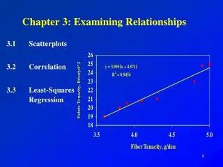
Unit 4/ Chapter 3 3-2 Least Squares Regression. Examining Relationships. Least-Squares Regression. When a scatterplot shows a linear relationship, we would like to summarize the overall pattern by drawing a line on the scatterplot.

E N D
Unit 4/ Chapter 3 3-2 Least Squares Regression Examining Relationships
Least-Squares Regression • When a scatterplot shows a linear relationship, we would like to summarize the overall pattern by drawing a line on the scatterplot.
Regression, unlike correlation, requires that we have an explanatory variable and a response variable.
Does fidgeting keep you slim? • Quickly review the example on Pg 200 Remember the toolbox... • Answer the key questions. • Graph the data • Calculate Numerical Summaries • Our new step.... Use a mathematical model to represent the data (we'll use a line!) • Interpretation
Does fidgeting keep you slim? • Here is the data and graph from the previous example.
Notice y = a + bx is the same model as the familiar y = mx + b from elementary algebra.
The Least-Squares Regression Line • So we want to draw a line as a model to represent our data (like density curves represented univariate data distributions in the previous chapter.) • But no line will go through all the points and my line drawn by eye might be different than yours • so...
The Least-Squares Regression Line(the LSRL) • ...find the line that reduces the vertical distances (squared so we don't deal with negatives) from the point to the line.
Using the LSRL • Given a LSRL, we want to be able to interpret it and use it. • Interpreting the slope: The slope tells us what? • Interpreting the y-intercept: The y-intercept tells us what? On average, for every added calorie of NEA, fat gain goes down by 0.00344 kilograms. The y-intercept (3.505 kg) is the estimated fat gain if NEA does not change when a person overeats.
Using the LSRL for predictions • Use the graph to predict values. What is the fat gain for a person whose NEA increases by 400 calories? • Or use the equation to predict values. Plug 400 into the equation.
Using the LSRL for predictions • Use the LSRL to predict the fat gain for someone whose NEA increases by 1500 calories. Then interpret your results. • This example introduces us to....
Using your calculator See page 210 Finding the LSRL using technology • Computer output-- Find the regressions on the computer outputs below.
Finding the LSRL algebraically We use (y-hat) to show that the predicted value given by the line will differ from the actual y value of the data.
Finding the LSRL algebraically • Using the same data from the NEA example, our numerical summaries are: sx=257.66 calories sy=1.1389 kg • Then use the fact that the LSRL passes through a = 3.505 kg 2.388 = a + (-0.00344)(324.8) Sois our regression line!
Residuals • Recall that the vertical distances from the points to the least-squares regression line are as small as possible. • Because those vertical distances represent “left-over” variation in the response after fitting the regression line, these distances are called residuals.
Or in other words, the residuals are the distances from the points to the LSRL.
Calculating a Residual • One subject's NEA rose by 135 calories and he gained 2.7 kg of fat. The predicted gain for 135 calories from the regression equation is: • The residual for this subject is therefore: observed - predicted
Fat Gain & NEA (yet again!) • Here are the residuals for all 16 data values from the NEA experiment: • Although residuals can be calculated from any model that is fitted to the data, the residuals from the least-squares line have a special property: the sum of the least-squares residuals is always zero. (Try adding the numbers above- - they add up to zero!)
The line y=0 corresponds with the regression line, and also marks the mean of our residuals. The residuals plot magnifies the deviations from the line to make patterns easier to see.
Residual Plots • What to look for when examining a residual plot: 1. Residual plots should have no pattern.
Residual Plots • What to look for when examining a residual plot: • A curved pattern shows that the relationships may not be linear. • Increasing spread about the line as x increases indicates the prediction will be less accurate for larger x values. Similarly, decreasing spread indicates the prediction will be less accurate for smaller x values.
Residual Plots What to look for when examining a residual plot: 1. The residual plot should show no pattern. 2. The residuals should be relatively small in size.
What is a small residual? Find S on each of the outputs below. S is called the standard deviation of the residuals. or the standard error of the residuals. S is the typical size of a residual.
The role of r2 in regression • A residual plot is a graphical tool for evaluating how well a linear model fits the data. • Look at the residual plot first to see if a linear model is a good fit. • If the linear model is a good fit, then there is also a numerical quantity that tells us how well the LSRL does at predicting values of the response variable y. It is r2, the coefficient of determination.
r2is actually the correlation squared, but there's more to the story... The idea of r2 is this: how much better is the least-squares line at predicting responses y than if we just used the mean of the y’s? The role of r2 in regression
Is the LSRL better at predicting the data values than the mean? r2 tells us how much better. The role of r2 in regression Here's the line that represents the y mean of our data. Here's our LSRL
Here's the formula: Note: Remember we defined the variance back when we talked about standard deviation. r2 compares the variance from the mean (the SST part of the equation) with the residuals (the SSE part of the equation).
For example, if r2=0.606 (as it does in the NEA example), then about 61% of the variation in fat gain among the individual subjects is due to the straight-line relationship between fat gain and NEA. The other 39% is individual variation among subjects that is not explained by the linear relationship.
When you report a regression, give r2 as a measure of how successful the regression was in explaining the response. When you see a correlation, square it to get a better feel for the strength of the linear relationship.
The distinction between explanatory and response variables is essential in regression. In the regression setting you must know clearly which variable is explanatory! ReviewFacts About Least-Square Regression
There is a close connection between correlation and the slope of the LSRL. The slope is This equation says that along the regression line, a change of one standard deviation in x corresponds to a change of r standard deviations in y. ReviewFacts About Least-Square Regression
The least-squares regression line of y on x always passes through the point (mean of x values, mean of y values) ReviewFacts About Least-Square Regression
The correlation r describes the strength of a straight-line relationship. The square of the correlation, r2, is the fraction of the variation in the values of y that is explained by the least-squares regression of y on x. ReviewFacts About Least-Square Regression