Download
1 / 61
620 likes | 784 Views
SCI 200 Physical Science Lecture 9 Color Mixing. Rob Daniell July 28, 2011. Color Mixing. Gilbert & Haeberli: Physics in the Arts Chapter 7 Additive color mixing Chapter 8 Subtractive color mixing Supplementary materials:

E N D
SCI 200 Physical Science Lecture 9Color Mixing Rob Daniell July 28, 2011
Color Mixing • Gilbert & Haeberli: Physics in the Arts • Chapter 7 Additive color mixing • Chapter 8 Subtractive color mixing • Supplementary materials: • Malacara, Daniel: Color Vision and Colorimetry: Theory and Applications,SPIE Press, Bellingham, 2001 • Wikipedia articles on Hue, sRGB, & ITU Recommendation 709 (Rec. 709) SCI200 - Lecture 10
Color Mixing • Trichromacy allows fairly strong hue discrimination • Nevertheless: • The same hue can be produced by different spectral distributions • Response of cones to any particular spectral distribution of light is complex • Is there a (relatively) simple way to describe or specify a particular hue? SCI200 - Lecture 10
Spectral Response of Cones • Two laser pointers (left) at 532 nm and 633 nm give the same hue as a single laser pointer (right) at 570 nm • Note that the authors seem to ignore the 2 pulses in the Type II cone produced by the 633 nm light • Gilbert & Haeberli, Physics in the Arts, pp. 86-87. SCI200 - Lecture 10
Idealized Color Wavelength Ranges • Gilbert & Haeberli, Physics in the Arts, p. 83. 600-700 nm 500-600 nm 400-500 nm SCI200 - Lecture 10
Color Mixing • Additive mixing • Two light sources • Combined by adding the intensity at each wavelength • Subtractive mixing • Filters, paints, dyes • Combined effect is produced by subtracting colors • Also depends on the light source SCI200 - Lecture 10
Additive Color Mixing • (a), (b), & (c): three non-monochromatic light sources • (d), (e), & (f): three two-color mixtures, each producing a third color • (g): spectral yellow • (h): unsaturated yellow produced by combining spectral green and spectral red • (i): the three non-spectral light sources mixed to produce white SCI200 - Lecture 10
Additive Color Mixing • (a): spectral blue + spectral yellow = white • Complementary colors • (b): broad band white • Mixture of many colors • metamers: Two different intensity distributions that appear the same to your eye SCI200 - Lecture 10
Additive Color Mixing • Additive color rules: • R + G + B =W • R + G =Y • G + B =C • R + B =M • Complementary colors: • R + C =W • G + M =W • B + Y =W • Can 3 colors be combined to produce any other color? C = Cyan, M = Magenta, Y = Yellow W = White SCI200 - Lecture 10
Additive Color Mixing • Red, Green, & Blue can be combined to produce most colors, but some saturated colors cannot be reproduced. • Red, Green, & Blue can be combined to produce more colors than any other choice of primary colors C = Cyan, M = Magenta, Y = Yellow W = White SCI200 - Lecture 10
Additive Color Mixing • CIE Color Matching experiments in 1922 • Illuminated region subtended a visual angle of 2° • Only the viewer’s fovea is illuminated • Matching field produced by 700 nm, 546.1 nm, 435.8 nm • Three spectral lines in mercury vapor SCI200 - Lecture 10
Additive Color Mixing • Hue, Saturation, and Luminance of the reference field were to be matched as closely as possible. • For some wavelengths (in fact, nearly all wavelengths) of the monochromatic source, a perfect match was impossible. • Except by adding one of the red, green, or blue matching colors to the reference field. SCI200 - Lecture 10
Additive Color Mixing • Suppose you attempt to match spectral cyan (490 nm) using • spectral red (650 nm) • spectral green (530 nm) • spectral blue (460 nm) • Spectral cyan produces • I: 1 pulse • II: 7 pulses • III: 2.5 pulses • spectral blue + spectral green produce • I: 2 + 0 = 2 1 • II: 2.5 + 16.5 = 19 9.5 • III: 1 + 9 = 10 5 SCI200 - Lecture 10
Additive Color Mixing • Spectral cyan: • I: 1 pulse • II: 7 pulses • III: 2.5 pulses • 50% blue + 36% green: • I: 1 + 0 = 1 • II: 1 + 6 = 7 • III: 0.5 + 3 = 3.5 • Spectral cyan + 33% red: • I: 1 + 0 = 1 • II: 7 + 0 = 7 • III: 2.5 + 1 = 3.5 • 50% blue + 36% green matches spectral cyan + 33% red SCI200 - Lecture 10
Additive Color Mixing • 50% blue + 36% green matches spectralcyan + 33% red • But spectralcyan + spectral red yields white: • So spectral cyan + 33% red is the same as 67% cyan + 33% white • That is, unsaturated cyan SCI200 - Lecture 10
Additive Color Mixing • Above: Spectral cyan on left; unsaturated cyan on the right • 50% blue + 36% green matches spectral cyan + 33% red • But spectral cyan + spectral red yields white: • So spectral cyan + 33% red is the same as 67% cyan + 33% white • That is, unsaturated cyan SCI200 - Lecture 10
Additive Color Mixing • Combine 460 nm (blue), 530 nm (green), and 650 nm (red) • To match the wavelength on the horizontal axis • Negative fractions mean you must ‘unsaturate’ the color you are trying to match • Standard observer: Based on data from 1931 SCI200 - Lecture 10
Additive Color Mixing • Previous figure redrawn so that complementary spectral colors lie opposite each other. • Saturated colors lie along the outside • Mixtures of two colors are proportional to the distance between them • along the line joining them • A line from one spectral color through the white point ends at the complementary color • White point depends on the precise standard used • The hue of the color at F is found by extending a line from white through F to the edge SCI200 - Lecture 10
Additive Color Mixing • International Commission for Illumination (CIE) • Did not want to use ‘negative colors’ to match saturated colors • Defined ‘imaginary colors’ [X], [Y], and [Z] • Not physical colors, but related • Defined ‘color matching functions’ x, y, and z • Relative amounts of [X], [Y], and [Z] needed to match a given spectral color (wavelength) • Results in “tristimulus” values x, y, and z • z = 1 - x - y • x and y together are called the ‘chromaticity’ of a color SCI200 - Lecture 10
Additive Color Mixing • CIE Chromaticity Diagram: • Horseshoe shaped curve represents saturated monochromatic colors • 380 nm - 700 nm • ‘purples’ (mixtures of blue and red) lie along bottom edge • z = 1 - x - y • Interior of horseshoe represents unsaturated colors SCI200 - Lecture 10
Additive Color Mixing • CIE Chromaticity Diagram: • Specify a color by three values • Chromaticity (x and y) • Lightness (or Brightness) • No representation is perfect • None can reproduce the precise color sensitivity of the human eye • Individual differences SCI200 - Lecture 10
Additive Color Mixing • RGB example: • 3 standard wavelengths: • 700 nm (red) • 546.1 nm (green) • 435.8 nm (blue) • These three colors can only reproduce colors in the interior of the triangle SCI200 - Lecture 10
Additive Color Mixing • CIE chromaticity diagram: • Three “primary” colors can only produce the colors inside the triangle - the “gamut” of the color set. • This triangle corresponds to the three colors used in a typical color monitor. SCI200 - Lecture 10
Additive Color Mixing • Monochromatic complementary pairs • 700 nm -- 494 nm • 600 nm -- 490 nm • 571 nm -- 380 nm • No complementary pairs between 494 nm & 571 nm SCI200 - Lecture 10
Additive Color Mixing • Color Triangle (Fig. 7.4) from textbook • Doesn’t cover gamut of the human eye • Does not conform to the sRGB standard used for color televisions and computer monitors • Does come close to maximizing the gamut of representable colors SCI200 - Lecture 10
Additive Color Mixing • Color Triangle inside a chromaticity diagram (Fig. 7.15) • It appears that the text uses • Red = 700 nm • Green = 530 nm • Blue = 440 nm • Does not conform to the “sRGB” standard for color television and computer monitors SCI200 - Lecture 10
Additive Color Mixing • sRGB standard • Based on 1931 CIE chromaticity • Red: x = 0.64, y = 0.33 • Green: x = 0.30, y = 0.60 • Blue: x = 0.15, y = 0.06 • White point: • x = 0.3127, y = 0.3290 • From the diagram, the dominant wavelengths are • Red: 611 nm • Green: 549 nm • Blue: 464 nm From Wikipedia http://en.wikipedia.org/wiki/Rec._709 SCI200 - Lecture 10
Additive Color Mixing • AdobeRGBstandard • Based on 1931 CIE chromaticity • Red: x = 0.64, y = 0.33 • Green: x = 0.21, y = 0.71 • Blue: x = 0.15, y = 0.06 • White point: • x = 0.3127, y = 0.3290 • From the diagram, the dominant wavelengths are • Red: 611 nm • Green: 535 nm • Blue: 464 nm • Green point is main difference with sRGB From Wikipedia http://en.wikipedia.org/wiki/Rec._709 SCI200 - Lecture 10
Additive Color Mixing • Complementary Colors to the “line of purples” appear to range from c491 nm to c579 nm SCI200 - Lecture 10
Additive Color Mixing • correspondence between wavelength and hue (angle): • complicated SCI200 - Lecture 10
Additive Color Mixing • correspondence between RGB and hue (angle): SCI200 - Lecture 10
Additive Color Mixing • LEDs approximate monochromatic red, green and blue: • Red = 645 nm • Green = 510 nm • Blue = 465 nm SCI200 - Lecture 10
Additive Color Mixing • LEDs approximate monochromatic red, green and blue: • Red = 645 nm • Green = 510 nm • Blue = 465 nm SCI200 - Lecture 10
Additive Color Mixing Methods • Methods and Techniques • Simple addition • Two or more light sources • Stage lights • Partitive mixing • Separate sources close to each other • Television screens & CRT displays • LCD displays • Rapid succession • Uses persistence of vision SCI200 - Lecture 10
Subtractive Color Mixing • Subtractive color combination: • Filters that absorb or block light of certain colors • Ink or pigments that reflect only certain colors and absorb the others • Primary Subtractive Colors: • Cyan, Magenta, Yellow • Supplemented by Black in “four color printing” C = Cyan, M = Magenta, Y = Yellow SCI200 - Lecture 10
Subtractive Color Mixing: Idealized Filters Idealized Blue Filter Idealized Green Filter Idealized Red Filter SCI200 - Lecture 10
Subtractive Color Mixing: Idealized Filters = “black” (no transmission) + Idealized Green Filter Idealized Red Filter SCI200 - Lecture 10
Subtractive Color Mixing: Idealized Filters Idealized Cyan Filter (blocks Red) Idealized Magenta Filter (blocks Green) Idealized Yellow Filter (blocks Blue) SCI200 - Lecture 10
Subtractive Color Mixing: Idealized Filters Idealized Cyan Filter + Idealized Magenta Filter = Blue filter SCI200 - Lecture 10
-R -G -B Subtractive Color Mixing: Block Diagrams • Subtractive Primaries: • C =B + G = W - R • M =B + R = W - G • Y =G + R = W - B SCI200 - Lecture 10
-R -G -R -B -G -B -R -G -B Subtractive Color Mixing: Block Diagrams • Basic Subtractive Rules: • C + M = B • C + Y = G • M + Y = R • C + M + Y = Bk (Black) SCI200 - Lecture 10
Subtractive Color Mixing • Dyes & Pigments: • Chemicals that absorb and/or reflect selective parts of the visible spectrum • Ideal dyes & pigments follow the same rules as ideal filters (i.e., subtractive color mixtures) • Real filters, dyes, and pigments often behave in complicated and (almost) unpredictable ways. SCI200 - Lecture 10
Subtractive Color Mixing • Real filters, dyes & pigments: • Usually smooth “corners” • Sometimes complicated structure • Rarely achieve trans-missions and reflectances of 100% SCI200 - Lecture 10
Subtractive Color Mixing • Real filters, dyes & pigments: • Can produce unexpected results The transmission of two or more filters in series is the product of the transmissions of each individual filter. For example: one filter with 70% transmission combined with another filter with 50% transmission produces a combined transmission of 35% 1 filter 2 identical filters 10 identical filters SCI200 - Lecture 10
Subtractive Color Mixing • Real filters, dyes & pigments: • Can produce unexpected results Combining filters or dyes with different transmittance functions can result in startling color shifts. yellow dye blue dye one-to-one mixture SCI200 - Lecture 10
reflectance of a magenta object cool white flourescent bulb resulting intensity distribution, the product of (a) and (b). Subtractive Color Mixing With subtractive colors the perceived color depends on the light source SCI200 - Lecture 10
Subtractive Color Mixing With subtractive colors the perceived color depends on the light source (example 2) a brown object a gray object In sunlight, the two objects at right have very different colors. Under an incandescent bulb, which emits much less blue light, the objects have very similar colors. SCI200 - Lecture 10
Subtractive Color Mixing Different light sources have different intensity distributions: Incandescent light bulb Deluxe Warm White Fluorescent bulb High Pressure Sodium Lamp SCI200 - Lecture 10
Subtractive Color Mixing Gamut of subtractive primaries: Gamut of color TV or computer monitor: Gamut of color slides: SCI200 - Lecture 10
Subtractive Color Mixing Printing inks: color is due to a combination of reflection and transmission: SCI200 - Lecture 10