Download

1 / 49
490 likes | 623 Views
College of Education and Health Professions. Basic Concepts. Chapter 1. Statistical Inference. A Population is a group with a common characteristic. A population is usually large and it is difficult to measure all members.

E N D
College of Education and Health Professions Basic Concepts Chapter 1
Statistical Inference • A Population is a group with a common characteristic. • A population is usually large and it is difficult to measure all members. • To make inference about a population we take a representative sample (RANDOM). • In a random sample each member of the population is equally likely to be selected. • A sample cannot accurately represent the population unless it is drawn without BIAS. • In a bias free sample selection of one member does not affect to selection of future subjects.
Types of Variables • Continuous variable – can assume any value (ht, wt) • Discrete variable – limited to certain values: integers or whole numbers (2.5 children?)
Level of Measurement • Nominal Scale: mutually exclusive (male, female) • Ordinal Scale: gives quantitative order to the variable, but it DOES NOT indicate how much better one score is than another (pain of 2 is not twice of 1) • Interval Scale: has equal units and zero is not an absence of the variable (temperature) • Ratio Scale: based on order, has equal distance between scale points, and zero is an absence of value
Independent & Dependent Variables • Independent Variable: the variable being controlled (gender, group, class). • Dependent Variable: NOT free to vary (math score, height, weight). • The INDEPENDENT VARIABLE is controlled by the researcher • Effects of exercise on body fat. • Effects of type of instruction on learning. • The DEPENDENT VARIABLE is the variable being studied • Body fat • learning
Parameters and Statistics • A parameter represents the population μ. • A statistic represents the sample . • The difference between a statistic and a parameter is the result of sampling error.
College of Education and Health Professions Describing and Exploring Data Chapter 2
A frequency distribution organizes the data in a logical order. Most of the scores are between 46 – 67.
Measures of Central Tendency • Mean, Median and Mode • Describe the middle or central characteristics of the data. • The mode is the most frequent score. • The median is the middle score. • In a normal distribution the mean, median and mode are the near the same score.
Measures of Variability • Range (lowest-highest). Suffers reliance on extreme scores. • Interquartile Range: middle 50% of the scores. • Variance: sum of squared deviations from the mean divided by (N-1), [data in squared units] • Standard Deviation: square root of the variance [data in original units].
Formulas for Mean, Variance and SD Standard Deviation Variance Mean
Degrees of Freedom • Df is the number of things that are free to vary. • For Example • The sum of three numbers is 10. The df is two, you can pick any two numbers. Once you pick the first two numbers the third number is fixed, it is not free to vary. 5 + 4 + ? = 10
SPSS Box Plots • The top of the box is the upper fourth or 75th percentile. • The bottom of the box is the lower fourth or 25th percentile. • 50 % of the scores fall within the box or interquartile range. • The horizontal line is the median. • The ends of the whiskers represent the largest and smallest values that are not outliers. • An outlier, O, is defined as a value that is smaller (or larger) than 1.5 box-lengths. • An extreme value, E, is defined as a value that is smaller (or larger) than 3 box-lengths. • Normally distributed scores typically have whiskers that are about the same length and the box is typically smaller than the whiskers.
A normal distribution is symmetrical, uni-modal and mesokurtic. Playturtic is flat. Leptokurtic is peaked.
Tests for Normality • Not less than 0.05 so the data are normal.
Tests for Normality: Normal Probability Plot or Q-Q Plot • If the data are normal the points cluster around a straight line
Tests for Normality: Boxplots • Bar is the median, box extends from 25 – 75th percentile, whiskers extend to largest and smallest values within 1.5 box lengths • Outliers are labeled with O, Extreme values are labeled with a star
College of Education and Health Professions Outliers and Extreme Scores Chapter 2
SPSS – Explore BoxPlot • The top of the box is the upper fourth or 75th percentile. • The bottom of the box is the lower fourth or 25th percentile. • 50 % of the scores fall within the box or interquartile range. • The horizontal line is the median. • The ends of the whiskers represent the largest and smallest values that are not outliers. • An outlier, O, is defined as a value that is smaller (or larger) than 1.5 box-lengths. • An extreme value, E , is defined as a value that is smaller (or larger) than 3 box-lengths. • Normally distributed scores typically have whiskers that are about the same length and the box is typically smaller than the whiskers.
Decisions for Extremes and Outliers • Check your data to verify all numbers are entered correctly. • Verify your devices (data testing machines) are working within manufacturer specifications. • Use Non-parametric statistics, they don’t require a normal distribution. • Develop a criteria to use to label outliers and remove them from the data set. You must report these in your methods section. • If you remove outliers consider including a statistical analysis of the results with and without the outlier(s). In other words, report both, see Stevens (1990) Detecting outliers. • Do a log transformation. • If you data have negative numbers you must shift the numbers to the positive scale (eg. add 20 to each). • Try a natural log transformation first in SPSS use LN(). • Try a log base 10 transformation, in SPSS use LG10().
Add 10 to the data. Then log transform. Add 10 to each data point. Try Natural Log. Last option, use Log10.
Add 10 to each data point, since you can not take a log of a negative number.
Outlier Criteria: 1.5 * Interquartile Range from the Median Milner CE, Ferber R, Pollard CD, Hamill J, Davis IS. Biomechanical Factors Associated with Tibial Stress Fracture in Female Runners. Med Sci Sport Exer. 38(2):323-328, 2006. Statistical analysis. Boxplots were used to identify outliers, defined as values >1.5 times the interquartile range away from the median. Identified outliers were removed from the data before statistical analysis of the differences between groups. A total of six data points fell outside this defined range and were removed as follows: two from the RTSF group for BALR, one from the CTRL group for ASTIF, one from each group for KSTIF, and one from the CTRL group for TIBAMI.
Outlier Criteria: 1.5 * Interquartile Range from the Median (using SPSS)
Outlier Criteria: 1.5 * Interquartile Range from the Median (using SPSS) Outliers = 1.5 * 3.39 above and below -.3549
Outlier Criteria: ± 3 standard deviations from the mean Tremblay MS, Barnes JD, Copeland JL, Esliger DW. Conquering Childhood Inactivity: Is the Answer in the Past? Med Sci Sport Exer. 37(7):1187-1194, 2005. Data analyses. The normality of the data was assessed by calculating skewness and kurtosis statistics. The data were considered within the limits of a normal distribution if the dividend of the skewness and kurtosis statistics and their respective standard errors did not exceed ± 2.0. If the data for a given variable were not normally distributed, one of two steps was taken: either a log transformation (base 10) was performed or the outliers were identified (± 3 standard deviations from the mean) and removed. Log transformations were performed for push-ups and minutes of vigorous physical activity per day. Outliers were removed from the data for the following variables: sitting height, body mass index (BMI), handgrip strength, and activity counts per minute..
Computing and Saving Z Scores Check this box and SPSS creates and saves the z scores for all selected variables. The z scores in this case will be named zLight1…
Computing and Saving Z Scores Now, you can identify and remove raw scores above and below 3 sds if you want to remove outliers.
Comparison of Outlier MethodsMedian ± 1.5 * Interquartile Range27 ± 1.5 * 7 gives a range of 16.5 – 37.5
Comparison of Outlier Methods± 2 SDs (Notice the 16’s are not removed)
Comparison of Outlier Methods± 2 SDs (Notice the 16s are not removed)
Comparison of Outlier Methods± 3 SDs (Step 1, then run Z scores again)
Comparison of Outlier Methods± 3 SDs (Step 2, after already removing the -44, the -2 then has a SD of -4.68 so it is removed)
Conclusions? • The median ± 1.5 * interquartile range appears to be too liberal. • ± 2 SDs may also be too liberal and statisticians may not approve. • An iterative process where you remove points above and below 3 SDs and then re-check the distribution may be the most conservative and acceptable method. • Choosing 3.1, 3.2, or 3.3 as a SD increases the protection against removing a score that is potentially valid and should be retained.
Decisions for Extremes and Outliers • Check your data to verify all numbers are entered correctly. • Verify your devices (data testing machines) are working within manufacturer specifications. • Use Non-parametric statistics, they don’t require a normal distribution. • Develop a criteria to use to label outliers and remove them from the data set. You must report these in your methods section. • If you remove outliers consider including a statistical analysis of the results with and without the outlier(s). In other words, report both, see Stevens (1990) Detecting outliers. • Do a log transformation. • If you data have negative numbers you must shift the numbers to the positive scale (eg. add 20 to each). • Try a natural log transformation first in SPSS use LN(). • Try a log base 10 transformation, in SPSS use LG10().