WORKSHOP 7 TAPERED PLATE

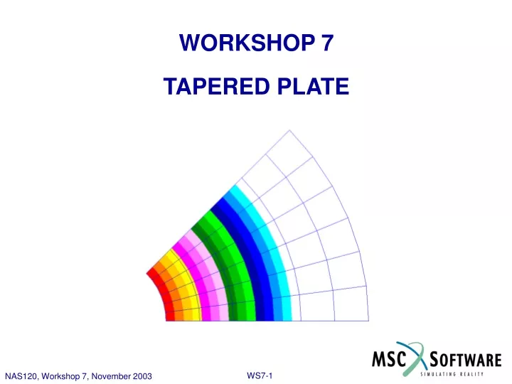
1. WORKSHOP 7 TAPERED PLATE WS7-1 NAS120, Workshop 7, November 2003

3. Problem Description Model a tapered annular plate with a variable pressure loading. Due to symmetry, only a 45° slice of the plate will be modeled. The plate is constructed from two different materials as shown below: Outer Region Aluminum Inner RegionSteel

4. Problem Description (cont.) The thickness variation in the plate is shown below:

5. Problem Description (Cont.) Table 8.1 Mesh Definition Table 8.2 Material Properties:

6. Workshop Objectives: • Learn to use fields to define element thickness • Learn to use fields to create variable pressure loading

7. Suggested Exercise Steps: • Create geometry representing a 45° slice of the annular plate. • Create the finite element mesh using the information listed in Table 12.1. • Create a cylindrical coordinate system. • Using the cylindrical coordinate system, define a spatially varying field which represents the plate thickness. Verify the field by creating an XY-plot. • Define material properties using the material constants shown in Table 12.2.

8. Suggested Exercise Steps: • Define element properties by assigning the material type and element thickness to the correct region of the model. • Verify that the spatial variation of the element thickness has been assigned correctly to the model by creating a scalar plot. • Define a spatially varying field that represents the pressure load. • Apply the pressure load. • Verify that the pressure has been assigned correctly by modifying plot markers.

9. Create a New Database • Create a new database called annular_plate.db • File / New. • Enter tapered_plate as the file name. • Click OK. • Choose Default Tolerance. • Select MSC.Nastran as the Analysis Code. • Select Structural as the Analysis Type. • Click OK.

10. Step 1. Geometry: Create/Curve/2D ArcAngles f • Create a curve • Geometry: Create / Curve / 2D ArcAngles. • Enter 1.0 for the Radius. • Enter 0.0 for Start Angle and 45 for End Angle. • Enter [0 0 0] for the Center Point List. • Click Apply. • Click on the Show Labels Icon. a b c d e

11. Step 1. (Cont.) Geometry: Create/Curve/2D ArcAngles • Create two more curves. • Enter 3.0 for the Radius. • Click Apply. • Enter 4.0 for the Radius. • Click Apply. c a b d

12. Step 1. (Cont.) Create/Surface/Curve • Create two surfaces. • Create / Surface / Curve. • Select 2 Curve for the Option. • Screen pick Curve 1, then Curve 2. A surface is automatically generated. • Screen pick Curve 2, then Curve 3. A second surface is generated. a b d c

13. Step 2. Finite Elements: Create/Mesh/Surface g • Mesh the two surfaces. • Finite Element: Create / Mesh / Surface. • Select IsoMesh as the Mesher. • Select Quad4 Element Topology. • Select both surfaces for the Surface List. • Enter 0.5 as the Global Edge Length. • Click Apply. • Click on Hide Labels icon. a b c d e f

14. Step 2. (Cont.) Finite Element: Equivalence /All/Tolerance Cube • Merge all coincident nodes. • Equivalence / All / Tolerance Cube. • Click Apply. a b

15. Step 3. Create/Coord/3Point • Create a cylindrical coordinate system. • Geometry: Create / Coord / 3 Point • Select Cylindrical as the type of coordinate system. • Enter [0 0 0] for origin, [0 0 1] for Point on Axis 3, and [1 0 0] for Point on Plane 1-3. • Click Apply. a b c d

16. Step 4. Fields: Create /Spatial/ Tabular Input • Create a field which defines the variation in plate thickness. • Fields: Create / Spatial / Tabular Input. • Type in thickness_spatial for the Field Name. • Select Coord 1 for Coordinate System. • Select R as the Active Independent Variable. • Click on the Input Data button to bring up the 1D Scalar Table Data window. • Enter the values into the table using the Enter key on the keyboard. Use the values shown on this page. • Click OK to return to the main field menu. • Click Apply. a f b c d g e h

17. Step 4. (Cont.) Field: Show • Verify the field using an XY plot. • Show. • Select thickness_spatial in the Select Field to Show window. • Click on the Specify Range button. • Check the Use Existing Points option. • Click OK to return to the main field menu. • Click Apply. a d b c e f

18. Step 5. Materials: Create / Isotropic / Manual Input • Create a material property set for steel. • Materials: Create / Isotropic / Manual Input. • Enter steel as the Material Name. • Click on the Input Properties button. • Enter 30e6 for the Elastic Modulus. • Enter 0.3 for the Poisson Ratio. • Enter 0.0007324 for the Density. • Click OK. • Click Apply. a d e f b c g h

19. Step 5. (Cont.) Materials: Create / Isotropic / Manual Input • Create a material property set for aluminum. • Materials: Create / Isotropic / Manual Input. • Enter alum as the Material Name. • Click on the Input Properties button. • Enter 10e6 for the Elastic Modulus. • Enter 0.33 for the Poisson Ration. • Enter 0.0002588 for the Density. • Click OK. • Click Apply. a d e f b c g h

20. Step 6. Element Properties: Create / 2D / Shell • Define Element Properties for the inner portion of the plate. • Properties: Create / 2D / Shell. • Enter prop_1 as the Property Set Name. • Click on the Input Properties button. • Click on the Select Material Icon. • Click on the steel in the Select Material window. • Change the thickness option from Real Scalar to Element Nodal. • Click on the Select Field Icon. • For the Thickness, select thickness_spatial from the Field Definitions section. • Click OK. • Select the inner surface for the Application Region. • Click Add. • Click Apply. a d f g b c j i k l e h

21. Step 6. (Cont.) Element Properties: Create / 2D / Shell • Define Element Properties for the outer portion of the plate. • Properties: Create / 2D / Shell. • Enter prop_2 as the Property Set Name. • Click on the Input Properties button. • Click on the Select Material Icon. • Click on the alum in the Select Material window. • Change the thickness option from Real Scalar to Element Nodal. • Click on the Select Field Icon. • For the Thickness, select thickness_spatial from the Field Definitions section. • Click OK. • Select the outer surface for the Application Region. • Click Add. • Click Apply. a d f g b c j i k l h e

22. Step 7. Element Properties: Show • Verify element properties using a scalar plot of the thickness. • Properties: Show. • Select Thickness from the Existing Properties window. • Select Scalar Plot as the Display Method. • Select Default Group. • Click Apply. a b c d e

23. Step 8. Fields: Create /Spatial/ Tabular Input Create a field which defines the variation in pressure. • Fields: Create / Spatial / PCL Function. • Type in pressure_variation for the Field Name. • Select Coord 1 for Coordinate System. • Enter the function: 100*’R. • Click Apply. a b c d e

24. Step 9. Loads/BCs: Create /Pressure/ Element Uniform Create a pressure load. • Loads/BCs: Create / Pressure / Element Variable. • Type in press for the New Set Name. • Set the Target Element Type to 2D. • Click Input Data. • Click on the Bottom Surf Pressure list box and select the field pressure_variation. • Click OK. a e b c f d

25. Step 9. Loads/BCs: Create /Pressure/ Element Uniform a Select an application region. • Click on the Iso 3 View Icon. • Click Select Application Region. • For the Geometry Filter select Geometry. • Select the Surface or Face filter. • Click in the application region list box and select both surfaces. • Click Add. • Click OK. • Click Apply. c d e f g b h

26. Step 10. Modify Plot Markers a h d i Modify the pressure plot markers. • Display: Load/BC/Elem.Props. • Select Show on FEM only. • Click on Vectors/Filters. • Change the length to Scaled- Screen Relative. • Click Apply. • Click Cancel. • Click on Label Style. • Set the Label Format to Integer. • Click OK. • Click Apply. b c g e f j

27. Step 10. Modify Plot Markers Re-plot the pressure plot markers. • Loads/BCs: Plot Markers. • Select the pressure load set. • Click Apply. a b c