Download
1 / 1
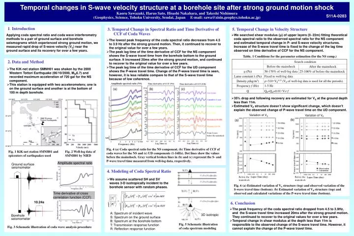
10 likes | 161 Views
1 . Introduction. 3. Temporal Change in Spectral Ratio and Time Derivative of CCF of Coda Waves. 2. Data and Method. Variation of V S. (b). Variation of V P. (a). Amplitude spectral ratio. Ground surface seismometer. Before the mainshock. Before the mainshock.

E N D
1. Introduction 3. Temporal Change in Spectral Ratio and Time Derivative of CCF of Coda Waves 2. Data and Method Variation of VS (b) Variation of VP (a) Amplitude spectral ratio Ground surface seismometer Before the mainshock Before the mainshock Time derivative of cross correlation function (CCF) 10.24s 3D isotropic Borehole seismometer Temporal changes in S-wave velocity structure at a borehole site after strong ground motion shock Kaoru Sawazaki, Haruo Sato, Hisashi Nakahara, and Takeshi Nishimura (Geophysics, Science, Tohoku University, Sendai, Japan E-mail: sawa@zisin.geophys.tohoku.ac.jp) S11A-0283 5. Temporal Change in Velocity Structure Applying coda spectral ratio and coda wave interferometry methods to a pair of ground surface and borehole seismograms which experienced strong ground motion, we measured rapid drop of S-wave velocity (VS) near the ground surface and its recovery for over a few years. • We searched shear modulus (μ)of upper layers (0~22m) fitting theoretical coda spectral ratio to the observed spectral ratio for the NS component and estimated temporal change in P- and S-wave velocity structures. Increase of the S-wave travel time is fixed to the change of the lag time observed on time derivative of CCF for the NS component. • The lowest peak frequency of the coda spectral ratio decreases from 4.5 to 3.9 Hz after the strong ground motion. Then, it continued to recover to the original value for over a few years. • The peak lag time of the time derivative of CCF for the NS component shows the S-wave travel time from the borehole bottom to the ground surface. It increased 20ms after the strong ground motion, and continued to recover to the original value for over a few years. • The peak lag time of the time derivative of CCF for the UD componentshows the P-wave travel time.Change of the P-wave travel time is seen, however, it is less reliable compare to that of the S-wave travel time because of low coherence. Table. 1 Conditions for the parameter estimation (for the NS comp.) • The KiK-net station SMNH01 was shaken by the 2000 Western Tottori Earthquake (06/10/2000, MW6.7) and recorded maximum acceleration of 720 gal for the NS component. • This station is equipped with two accelerometers; one is on the ground surface and another is at the bottom of 100 m depth borehole. (a) (b) (c) • 35% drop and following recovery are estimated for VS at the ground depth less than 11m. • Estimated VP structure doesn’t show significant change, which doesn’t explain the observed change of P-wave travel time on the UD component. Fig. 4 (a) Coda spectral ratio for the NS component. (b) Time derivative of CCF of coda waves for the NS and (c) UD components (1-16Hz). Dot lines show the values before the mainshock. Gray vertical broken lines in (b) and (c) represent the S- and P-wave travel time measured from well-log data, respectively. Fig. 1 KiK-net station SMNH01 and epicenters of earthquakes used Fig. 2 Well-log data of SMNH01 by NIED 4. Modeling of Coda Spectral Ratio • We assume scattered SH and SV waves 3-D isotropically incident to the borehole sensor with random phases. Fig. 6 (a) Estimated variation of VS structure (top) and observed variation of the S-wave travel time (bottom). (b) Estimated variation of VP structure (top) and observed and calculated variations of the P-wave travel time (bottom). 6. Conclusion • The peak frequency of the coda spectral ratio dropped from 4.5 to 3.9Hz, and the S-wave travel time increased 20ms after the strong ground motion. They continued to recover to the original values for over a few years. • Temporal change in shear modulus at the depth less than 11m is responsible to the observed change of the S-wave travel time. However, it cannot explain the change of the P-wave travel time. A: Spectrum of incident wave S: Spectrum on the ground surface B: Spectrum at the borehole bottom T: Transmission response function R: Reflection response function Fig. 5 Schematic illustration of coda spectrum modeling Fig. 3 Schematic illustration of coda wave analysis procedure