Download
1 / 21
210 likes | 266 Views
Lecture 12: The beautiful theory of interferometry. First, some movies to illustrate the problem. Clues of what sort of maths to aim for. Geometrical calculation of phase. Visibility formulas. Simplifying approximations:.

E N D
Lecture 12:The beautiful theory of interferometry. • First, some movies to illustrate the problem. • Clues of what sort of maths to aim for. • Geometrical calculation of phase. • Visibility formulas.
Simplifying approximations: • I’ll assume a small bandwidth Δν, so signals can be approximated by sinusoids. • I’ll neglect polarization. • I’ll explain interferometry first in 2 dimensions, then extend this to 3. • There are many sorts of interferometer but I’ll concentrate on aperture synthesis. • The fundamental maths for a 2-antenna interferometer can be easily expanded to cater for more than 2.
Expression for the phase difference φ Path difference d = D sinθ θ D=uλ
Clues..? • Since φ is proportional to sin(θ), if we could measure φ, we could work out where the source is in the sky. • From last lecture, we saw that correlating the signals from the two antennas gives us a number proportional to S exp(-iφ), where S is the flux density of the source in W Hz-1. Things are looking good! • The fly in the ointment is...
The sky is full of sources. The correlation returns an intensity-weighted average of all their phases. D=uλ
Formally speaking... • The correlation between the voltage signals from the two antennas is • We’ll call V the visibility function. • A is the variation in antenna efficiency with θ. • I is the quantity formerly known as B – ie the brightness distribution. Its units (in this 2-dimensional model) are W m-2 rn-1 Hz-1 • To keep things simple(r) I’ve ignored any summation over frequency ν.
Coordinate systems – everything is aligned with the phase centre. For baselines: w u dθ l =sinθ (1-l2)1/2 Celestial sphere =cosθ θ The direction normal to the plane of the antennas is called the phase centre. Normally the antennas are pointing that way, too. 2 1 b
Putting it all together: • gives • We want to complete the change of variable from θ to l. It’s not hard to show that • so the final expression is
Ahah! • Provided w=0, or in other words provided the antennas all lie in a single plane normal to the phase centre, • This is a Fourier transform! We just need to get a lot of samples of V at various u, then back-transform to get • Trouble is, we can’t always keep w=0.
Non-coplanar arrays. For baselines: w u dθ l Phase centre (1-l2)1/2 θ 2 1 u1,3 b1,2 w1,3 = w2,3 b1,3 b2,3 3
Non-coplanar arrays - small-field approximation: • The factor of (1-l2)1/2 prevents the full expression for V´(u,w) from being a Fourier transform. • But for small l, (1-l2)1/2 is close to 1, and varies only slowly. Let’s do a Taylor expansion of it: • The full expression therefore becomes (1-l2)1/2 = 1 – ½l2+O(l4).
Non-coplanar arrays - small-field approximation: • For V(u)=V´(u,w)exp(2πiw), and πwl2<<1, and we are back to the Fourier expression. • V is like measuring V´ with a phantom antenna in the same plane as the others. • So: for non-coplanar antennas, what matters is the projection lengthu of each baseline, projected on a plane normal to the ‘phase centre’.
The phase centre • The location of the phase centre is controlled as follows: • Decide which direction you want to be the phase centre. • That direction defines the orientation of the u-w axes. • Calculate wj,k for each j,kth baseline in that coordinate system. • Multiply each correlation Rj,k by the appropriate e2πiw factor. (Equivalent is to delay the leading signal by t=w/ν.) • After appropriate scaling, the result is a sample of the visibility function V(uj,k) appropriate to the chosen phase centre.
Now we go to 3 dimensions and N antennas. • The coordinate axes in 3 dimensions are labelled (u,v,w) for baselines and (l,m,n) for source vectors. • Each pair of antennas gives us a different projected baseline. • N antennas give N(N-1)/2 baselines. • Thus N antennas give N(N-1)/2 samples of the ‘coplanar’ visibility function
An example The full visibility function V(u,v) (real part only shown). A familiar pattern of ‘sources’
Let’s observe this with three antennas: v Latitude u Longitude