Download
1 / 28
321 likes | 586 Views
Magneto-optical imaging of Superconductors. Satyajit S .Banerjee Dept of Physics, Indian Institute of Technology, Kanpur, India. Principle of operation of MO imaging. Faraday Effect:. F = V B z d. M. Light source. M. P. P. A. A. M. Polariser. Z. d. Analyser. X.

E N D
Magneto-optical imaging of Superconductors Satyajit S .Banerjee Dept of Physics, Indian Institute of Technology, Kanpur, India
Principle of operation of MO imaging • Faraday Effect: F = V Bz d M Light source M P P A A M Polariser Z d Analyser X Transmission Mode Z Y
Reflection Mode MO Polarized light F = V Bz 2d MO active layer GGG d M Reflecting layer Sample Protective layer Z Y X
Types of MO active layers • Type of MO active layer depends on the type of experiments. d YIG EuTe EuSe
MO imaging setup Choice YIG : For high magnetic field resolution and Wide T range of application Typical Faraday rotation: 0.06 deg/mT for 2-5 m thick indicators I=IoSin2(2VdBz) or I Bz2
Sensitivity of the MO technique • Field sensitivity is determined by the Faraday rotation 2Vd & noise For EuTe~20mT for Bi doped YIG ~ 0.15 mT • Spatial resolution Governed by thickness (d) + distance between sample and MO active layer (z) d z Sample
Sensitivity of the MO technique • Temporal resolution Governed by the Quantum efficiency and the minimum exposure time permissible by the imaging device like a video camera. Temporal resolution ~ at best a few mSecs In recent times there have been nearly two to three order of magnitude improvement in field, spatial and temporal resolution
a0~(0/B)1/2 At B = 1 T, a0~500 A0 ~ 5 x 10¹⁰ vortices/cm2 Some basic ideas about vortices 2~5-10 nm
Loss of sensitivity in resolving vortices with increasing dist. With increasing distance of the MO active layer from the surface of the superconductor causes loss of the resolving power for resolving vortices.
Applications of MO at Mesoscopic length scales Strong meissner screening currents on surface • Observing the Meissner effect in superconductors YBCO, 10 K, field of 10 G • Observing the Critical state YBCO, 70 K, field of 100mT B x 0
disordered ordered kBT solid liquid 213.2 213.1 213.0 Phase transitions in the vortex state Similarities between ice to water transition & Vortex solid to liquid transition 213.4 liquid vor B 213.3 B(G) B~0.2G B~0.1%B solid H = 240 Oe a 58.35 58.40 58.45 58.50 58.55 T [ K ]
»1 G B(x) Source of noise in MOI • Static: • Indicator inhomogeneities and defects • CCD pixel variations • Light inhomogeneities • Dynamic: • CCD noise • Light fluctuations • Vibrations • Fundamental noise: • Photon shot noise
n up n up Ha+Ha static noise Ha Ha n down n~10 …~100 times differential static noise Ha Differential MOI imaging • dc field B = 100 G • Equilibrium magnetization step B 0.1 G • Desired resolution ~0.01 G • Required signal/noise 100/0.01=104 • Photon shot noise N/N = (N)1/2 N=108 photons/pixel • CCD full well capacity ~105 electrons ~103 frames • Reduce static noise by differential process:
image A small large small F=B F P Difference image: temperature scan light source Solid (no change in B) 213.4 liquid 213.3 B(G) B~0.2G B~0.1%B 213.2 solid 213.1 Liquid change in B already occurred 213.0 H = 240 Oe a 58.35 58.40 58.45 58.50 58.55 MO indicator T [ K ] mirror N S Observation of melting in MOI Dept. of Condensed Matter Physics Weizmann Institute Of Science
5 1 0 4 1 0 3 1 0 2 1 0 1 1 0 0 2 0 4 0 6 0 8 0 1 0 0 Phase diagram of melting Hc2 liquid depinning solid disordered second magnetization peak B [G] first-order transition quasi-ordered-lattice (Bragg glass) T [K]
Columnar defects Effect of disorder on melting Sample Bi2Sr2CaCu2O8 (BSCCO), Tc ~ 89-90 K SST mask 90mm
Porous vortex solid Melting phase diagram in presence of disorder S. S. Banerjee et al, Phys. Rev. Lett. 90, 87004 (2003) Vortex Liquid ?
Fixed H,T (MO Image with I+) - (MO Image with I-) = Difference Image Schematic of self field image one should see Inversion scheme Wijngaarden et al PRB54, 6742 (96) Self field generated by I (Biot-Savarts law) Sample with uniform I distribution Can detect self field down to 0.1 mA Two to three orders of magnitude improvement in sensitivity Imaging transport current distribution using MOI S. S. Banerjee et al, Phys. Rev. Lett. 93, 97002 (2004)
Self-induced field Current distribution 30mA, 75K, 25G Some examples :Surface barrier - I - V + V + I 0.5mm BSCCO crystal
Imaging current distribution in the vortex liquid phase Unirradiated NL Irradiated S. S. Banerjee et al, Phys. Rev. Lett. 93, 97002 (2004)
GGG d M Reflecting layer Sample Micron-submicron resolution Prof. Tom Johansens Group, Oslo, Norway • Single vortex imaging with MO MO layer Conventional MO indicator: Protective layer Latest MO indicator: GGG M Sample
Interaction of magnetic Domain walls with vortices Dynamics of single vortices
Nanosecond temporal resolution Paul Leidere’s group, University of Konstadz, Germany
Application of MO in different areas of condensed matter physics L.E.Helseth et al, PRL 91, 208302 (2003) Manipulating magnetic beads Dilute magnetic semiconductors (Mn doped GaAs) U. Welp et al., PRL 90, 167206 (2003)
Summary • Two orders of magnitude improvements in spatial, temporal and magnetic field sensitivity. • Improvement in transport current detection capability • Enormous potential for investing the physics of magnetic response in a diverse class of materials.
Acknowledgements Prof Eli Zeldov, Israel Prof Yossi Yeshurun, Israel. Prof. Marcin Konczykowski,France Prof. Kees van der Beek, France Prof. Tsuyoshi Tamegai, Japan Prof. M. Indenbom, Russia Prof Tom Johansen, Oslo Prof. Paul Leiderer, Germany Prof. A. A. Polyanski, USA Prof. Vlasko Vlasov, USA Prof. U. Welp, USA Prof. Larbalestier, USA Prof. H. Brandt