Download

1 / 11
110 likes | 269 Views
CS 585 Computational Photography. Nathan Jacobs. so far we have been compositing by averaging the two images…. but that is not the only option. What about finding an optimal seam?. Davis, 1998. Segment the mosaic Single source image per segment Avoid artifacts along boundries

E N D
CS 585 Computational Photography Nathan Jacobs
so far we have been compositing by averaging the two images…
but that is not the only option What about finding an optimal seam?
Davis, 1998 • Segment the mosaic • Single source image per segment • Avoid artifacts along boundries • Dijkstra’s algorithm
2 _ = overlap error min. error boundary Minimal error boundary overlapping blocks vertical boundary
Beyond dynamic programming • What if we want similar “cut-where-things-agree” idea, but for closed regions? • Dynamic programming can’t handle loops • Why not? • What else can we do?
An aside: Binary Markov Random Field Unary terms (compatability of data with label y) Pairwise terms (compatability of neighboring labels) Subject to conditions on P there is an easy to use polynomial time algorithm for optimizing this cost function (graph cuts, Min cut/Max Flow). Useful to look at this as a graph (a CS graph). Slide by Simon Prince
Graph Construction • One node per pixel (here a 3x3 image) • Edge from source to every pixel node • Edge from every pixel node to sink • Reciprocal edges between neighbours Note that in the minimum cut EITHER the edge connecting to the source will be cut, OR the edge connecting to the sink, but NOT BOTH (unnecessary). Which determines whether we give that pixel label 1 or label 0. Now a 1 to 1 mapping between possible labelling and possible minimum cuts Slide by Simon Prince
a cut hard constraint n-links hard constraint t s Graph cuts (simple example à la Boykov & Jolly, ICCV’01) Minimum cost cut can be computed in polynomial time (max-flow/min-cut algorithms)
Next Time • More on graph cut based methods: • Lazy Snapping • Grab Cut • Interactive Digital Photo Montage • Upcoming classes: • Monday: normal • Wednesday, Friday, then Monday, Wednesday: unclear (probably two days w/o class)