Download
1 / 18
180 likes | 345 Views
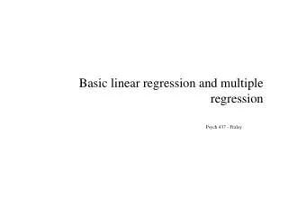
LESSON 6: FORECASTING TREND-BASED TIME SERIES METHODS. Outline Linear Regression Holt’s Method. Linear Regression. Linear regression is a useful tool that can provide relationship between two variables.

E N D
LESSON 6: FORECASTING TREND-BASED TIME SERIES METHODS Outline Linear Regression Holt’s Method
Linear Regression • Linear regression is a useful tool that can provide relationship between two variables. • When a scatter diagram shows that two variables are linearly or nearly linearly related, linear regression can provide a mathematical relationship between two variables. The relationship is expressed in terms of an equation. • Using linear regression, we can infer how good the relationship is.
Linear Regression • We discuss linear regression in three contexts: • Lesson 2: To estimate the learning curve parameters. This is the only context when we compute logarithms before using the method of regression. The reason for this is that u and Y(u) are not linearly related. However, log(u) and log(y(u)) are nearly linearly related. So, linear regression is used on log(u) and log(y(u)). • Lesson 6: To forecast demand from a known value of some other variable. • Lesson 7: To extend the deseasonalized demand series.
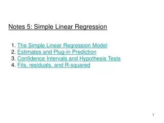
Y Dependent variable X Independent variable Linear Regression The scatter diagram on this slide shows a linear relationship between two variables.
Regression equation: Y = a + bX Y Dependent variable X Independent variable Linear Regression A straight line of the form Y = a+bx nicely fits the points. Linear regression can provide values of parameters a and b
Deviation, or error Regression equation: Y = a + bX Y Estimate of Y from regression equation { Actual value of Y Dependent variable Value of X used to estimate Y X Independent variable Linear Regression The least square method finds a and b such that the sum of the squares of errors is minimum
Sales Advertising Month (000 units) (000 $) 1 264 2.5 2 116 1.3 3 165 1.4 4 101 1.0 5 209 2.0 Linear Regression Future sales are unknown, but future advertising expenses may be known. A known value of advertising expense may provide a forecast of sales if we can find the relationship between these two variables. Since sales depends on advertising, sales is the dependent variable and shown on the y-axis. Advertising is the independent variable and shown on the x-axis.
Sales, y Advertising, x Month (000 units) (000 $) xyx 2 1 264 2.5 2 116 1.3 3 165 1.4 4 101 1.0 5 209 2.0 Total y= x = xy - nxy x 2 - nx 2 a = y – bx = b = = Linear Regression
300 — 250 — 200 — 150 — 100 — 50 Linear Regression Y = Interpretation: Sales (000s) | | | | 1.0 1.5 2.0 2.5
Linear Regression • Coefficient of correlation, r, provides information on how strong the relationship is.The formula for computing r is shown in the next slide. • The value of r varies from -1 to +1. • A negative value of r indicates a negative relationship (the regression line will have a slope downward to the right) and a positive value of r indicates a positive relationship (the regression line will have a slope upward to the right). • The value of r2 varies from 0 to 1. A value near 0 indicates a very weak or no relationship. A value near 1 indicates a very strong relationship.
Sales, y Advertising, x Month (000 units) (000 $) xyx 2y 2 1 264 2.5 660.0 6.25 2 116 1.3 150.8 1.69 3 165 1.4 231.0 1.96 4 101 1.0 101.0 1.00 5 209 2.0 418.0 4.00 Total 855 8.2 1560.8 14.90 y = 171 x = 1.64 nxy - x y [nx 2 -(x) 2][ny 2 - (y) 2] r = Linear Regression
Sales, y Advertising, x Month (000 units) (000 $) xyx 2y 2 1 264 2.5 660.0 6.25 69,696 2 116 1.3 150.8 1.69 13,456 3 165 1.4 231.0 1.96 27,225 4 101 1.0 101.0 1.00 10,201 5 209 2.0 418.0 4.00 43,681 Total 855 8.2 1560.8 14.90 164,259 y= 171 x = 1.64 r = 0.98, r 2 = 0.96 Since r = 0.98>0, relationship is positive Since r 2 = 0.961, relationship is very strong Linear Regression
Linear Regression The regression equation can be used to forecast sales of Month 6 from a known value of advertising expenditure in Month 6. Forecast for Month 6: Let advertising expenditure = $1750 Y =
Linear Regression 80 — 70 — 60 — 50 — 40 — 30 — Yn = a + bXn where Xn = Weekn Patient arrivals | | | | | | | | | | | | | | | 0 1 2 3 4 5 6 7 8 9 10 11 12 13 14 15 Week
Double Exponential SmoothingHolt’s Method • The method uses two smoothing constants and • The method iteratively computes St and Gt respectively slope and gradient at period t • Initial slope and gradient S0 and G0 are needed to start the computation • Finally, St and Gt can be used to obtain a -step ahead forecast, Ft,t+ from period t
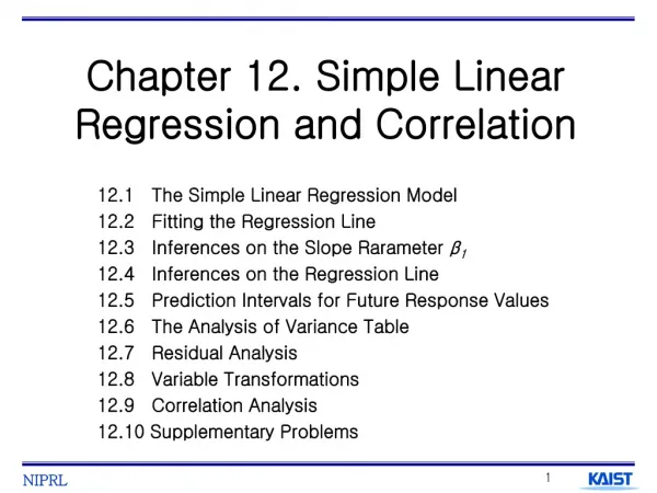
A Comparison of Methods 90 85 Actual 3-Mo MA 80 3-Mo WMA Demand 75 Exp Sm 70 Double Exp Sm 65 60 0 5 10 15 Months
READING AND EXERCISES Lesson 6 Reading: Section 2.8, pp. 77-81 (4th Ed.), pp. 74-77 (5th Ed.) Exercises: 28, 30, pp. 79, 81 (4th Ed.), pp. 75, 77 (5th Ed.)