Download
1 / 16
160 likes | 392 Views
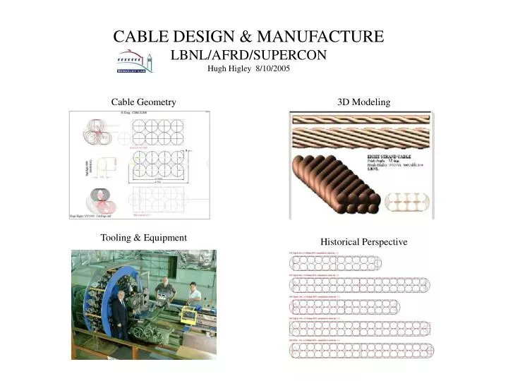
CABLE DESIGN & MANUFACTURE LBNL/AFRD/SUPERCON Hugh Higley 8/10/2005. Cable Geometry. 3D Modeling. Tooling & Equipment. Historical Perspective . CABLE DESIGN PHILOSOPHY .

E N D
CABLE DESIGN & MANUFACTURELBNL/AFRD/SUPERCONHugh Higley 8/10/2005 Cable Geometry 3D Modeling Tooling & Equipment Historical Perspective
CABLE DESIGN PHILOSOPHY • Rutherford cables are similar to other roll-formed, drawn or extruded products, in that a finished cable can be understood by modeling the deformation experienced during the cabling process. • A comparison between feed-stock and final-cable dimensions, gives insight to the strain and deformation introduce during cabling. To this end we must first have a description of the cable as feed stock prior to deformation, and then, an examination of the tooling and methods used to apply the deformation. • The delicate internal structures of superconducting wire impose limits to acceptable strain and deformation, in that superconductor performance falls off steeply once internal structures are damaged. Fundamentally, cable design parameters should not exceed a superconductor’s material limitations. • In an R&D environment it is important to limit known variables to those being tested, i.e. conductor performance vs. magnet performance and for this reason at LBNL a conservative approach to cable design has been chosen. Our design philosophy is to minimize superconductor degradation, preserving the conductor to magnet performance correlation. This means that we put a higher priority on delivering uniform quality cable with predictable properties than on maximizing cable current density.
Cable Design Parameters Modeling cable as feed stock is at first simple. Rutherford cables have a very uniform periodic structure. A cable’s geometry can be described using just a few equations, If first we assume there are no gaps between strands and we treat the wires as geometric entities, i.e. ignoring any material properties. The parameters needed to model cable are: Given: - Strand Diameter - Number of Strands - Cable Pitch-Angle Then: - Cable Thickness = 2 x Strand Dia. - Cable Pitch-Length = No. Strands x (Strand Dia. / SIN(Pitch-Angle) - Cable Width = ((No. Strands / 2) x (Strand Dia. / COS(Pitch-Angle))) + (0.732 x Strand Dia.)
Calculating Cable Pitch-Length (Strand Diameter / SIN(Pitch Angle_A) A Pitch Length = Number of Strands x (Strand Diameter / SIN(Pitch Angle_A)
Calculating Cable Width Cable Width = ((No. of Strands / 2) x (Strand Dia. / COS(Pitch Angle))) + (0.732 x Strand Dia.) -Example: 8-Strands, Dia.=1 Black and Red circles represent Min and Max Width phases along the cable. This drawing uses circles, so taking into account the COS(Pitch Angle) contribution, we get the equation above.
ODD vs. EVEN NUMBERS of STRANDS Correct 2D representation of odd strands. Incorrect 2D representation The case has been made by some, that there is an advantage to odd numbers of strands in a cable. I believe that this confusion comes from a misrepresentation of cable when drawn as 2D cross-sections. It is true that for even stranded cables the maximum width is reached at both edges simultaneously while odd numbered cables alternate from side to side. This does not mean that odd numbered cables have a more uniform distribution of widths. When viewed as 2D cross-sections it is easy to misalign the odd stranded cable between phases and come to the wrong conclusion that the width for odd stranded cables is more uniform. In the examples below red and black ellipses represent rotational phases along the cable. Same width in both phases is misleading
3D-Model Introduction In a geometric model of cable there is no strain, but in a real cable there is an initial or starting strain in the strands due to bending at the cable edges. In order to calculate the initial strain in the strands we need to know the bend radii, which requires three dimensional modeling. The starting assumptions for the 3D model are the same as before. If we assume that there are no gaps between strands and we treat the wires as geometric entities, i.e. ignoring any material properties. We then must account for the strands rotation about the length of the cable. I have assumed also that the strands move in a constant linear path across the width of the cable. The result of the two linear motions top and bottom is to drive individual strands around the edge through a non linear path in which the edge strand maintains contact with it’s neighbors.
3D Model Approach Before a 3D model could be constructed the centerline path for the strands was needed. An equation that integrates the linear path in the top and bottom with the nonlinear path at the cables edges would be ideal but so far I have only been able to use brute force via 2D analysis and successive approximations to approximate the coordinates of the centerline path. I have been able however to optimize a sub set of coordinates that are consistent to within (0.001 strand diameter) for the pitch angles of interest between 10 and 20deg.
Edge Geometry You can see from the illustration below that the strand at the edge (red) is driven around by the linear action of the upper and lower strands (black/green). The center-line path of the strand is an ellipse with proportions 1: 0.732.
3D Model Rendered It was then possible using CAD software to visualize the 3D centerline path for the strands in a cable. By “extruding” a wire along the centerline path, the observed fit between strands validated the 2D modeling effort.
3D Bend Radius With a validated 3D model it is possible to calculate the initial bend radius present in a cable before it is roll formed to final dimensions. The minimum bending radius prior to roll forming cable is 4.0 x Strand diameter.
3D Pitch angle 15º 24º For a cable with an assumed pitch angle across the cable width of 15deg, as in the drawing below, Top view the strand will reach a maximum pitch angle of ~24º at the cable edges. This means that while the strand cross-sectional area in the mid region increases by ~3.5%, in the edges strand cross-sectional area increases by ~9.5% Edge view
Packing Factors -Edge .361 Hugh Higley 10/17/2004 2D-Packing Factor [PF] at the cable edges is defined by the blue rectangle, known as an edge quadrant. - An edge quadrant is the smallest edge unit area that has the same ratio of strand area for all phases. Height = Strand Diameter Width = Strand Width + (0.361 x Strand Diameter) Strand Width = Strand Diameter / COS(Pitch Angle) PF = Strand Area / Rectangle Area x (StrandDia / 2) x (StrandDia / COS(PitchAngle)) / 2) StrandDia x [(StrandDia / COS(PitchAngle))+(0.361 x StrandDia)] = [ 58.23% ] The 3D model, which assumes constant pitch angle in the mid region, clearly shows that pitch angle increases significantly to a max of 24.0 through the edge region, or equivalent to 9.5% increase in cross-sectional area at edge maximum. The 3D PF would be somewhat greater than 58.23% (?) in the edge region when all phases are integrated. The measured 3D volumetric Packing Factor in an edge quadrant for a cable at 15º pitch is 62.98%
Packing Factors Mid Packing Factor in the cable center region is defined by the black rectangle. /4 = [ 78.54% ] Height = Strand Diameter Width = Strand Diameter / COS(Pitch Angle) PF = Strand Area / Rectangle Area x (StrandDia / 2) x (StrandDia / COS(PitchAngle)) / 2) StrandDia x (StrandDia / COS(PitchAngle)) While 2D packing factors and 3D packing factors are initially equivalent in the center region, this only holds true for the cable prior to deformation. Once deformation has begun, nonlinear 3D material- flow is expected.
NON LINEAR FLOW Flow Flow It is important to recognize that once deformation has begun in the 3D model the flow will be very non linear. By this I mean that 2D analysis will not suffice as there will also be material flow that is perpendicular to each wire. These strand perpendicular flows are not represented in any 2D cross-section of the cable. There is also a significant level of friction resisting strand-perpendicular flow at the roller surfaces while comparably sized load bearing interfaces between strands have relatively low resistance to strand perpendicular flow. This surface friction differential can concentrate or restrict flow in certain areas. For example, imagine a clear balloon with a small circle drawn on the surface. If the balloon is pressed against a hard surface with the circle at the interface you would see that the circle in question would expand less than comparable circles on the rest of the balloon due to friction supplied by the hard surface. Then If you imagined instead pressing two identical balloons together the circles at the interface would grow similarly to comparable circles elsewhere on the balloon. This analogy is useful in that when packing-factors are low and wires have line contact with there neighbors wire elongation is negligible wile surface flow perpendicular to the line contacts dominates. Flow Flow Flow Flow
Non linear flow Strands in the edge quadrants initially have only 2 line contacts with neighbors plus an intermittent point contact with a hard surface. While each wire in the center region initially has3 line contacts, one of witch is to a hard surface, plus intermittent point contactswith opposing strands. A strand and its opposing strand touch at 2x the pitch angle meaning that these opposing strand perpendicular flows are not parallel with each other, introducing a yet undefined friction. Add to this that superconducting strands are metallic composites with extremely anisotropic properties and come in infinite varieties of materials, and the modeling effort seems overwhelming with little certain payoff. Yet I believe that if we model a simple homogenous material like copper then we will be able make predictions about the locations of peak flow and the options available to control deformation. Then we will have a reference to measure the difference in behavior between predicted deformation and real deformation in a quantifiable framework.