Download
1 / 19
190 likes | 194 Views
Measuring Decision Weights for Unknown Probabilities by Means of Prospect Theory. Peter P. Wakker & Enrico Diecidue & Marcel Zeelenberg. Domain: Individual Decisions under Ambiguity (events with unknown prob s ; Keynes 1921, Knight 1921).

E N D
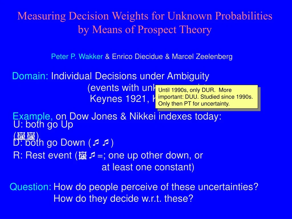
Measuring Decision Weights for Unknown Probabilities by Means of Prospect Theory Peter P. Wakker & Enrico Diecidue & Marcel Zeelenberg Domain: Individual Decisions under Ambiguity (events with unknown probs; Keynes 1921, Knight 1921) Until 1990s, only DUR. More important: DUU. Studied since 1990s. Only then PT for uncertainty. • Example, on Dow Jones & Nikkei indexes today: • U: both go Up () • D: both go Down () • R: Rest event (=; one up other down, or • at least one constant) Question: How do people perceive of these uncertainties? How do they decide w.r.t. these?
2 Knight (1921): Such uncertainties are “unmeasurable.” Famous result by de Finetti (1931): showed how to measure them after all.
U D R $7 $5 $9 ( ) 3 de Finetti’s (1931) book making: No book making ( no arbitrage) • People have to take subjective probabilities • U of U • D of D • R of R, • (nonnegative, U + D + R = 1) • and evaluate Impressive! Philosophers filled libraries … U7 + D5 + R9 by Obtains expected value = subj. exp. utility with linear utility. For moderate stakes, other factors than utility curvature are more important for understanding risk attitudes. Linear utility is reasonable for moderate stakes!
( ) = , • If ~ U D R U D R 1 0 0 ( ) 4 • In classical model, an easy way to elicit subj. probs: through betting odds on events. • thenU = . • However,Subj. Exp. Utty has descriptive problems(Ellsberg 1961). • Constructive alternative: Cumulative prospect theory(Tversky & Kahneman 1992). • Merges - original prospect theory (Kahneman & Tversky 1979) & - rank-dependent utility (Quiggin 1981, Schmeidler 1989).
U D R U D R ( ) U D R UUU 1 0 0 1 0 0 b b b ( ) U D R ~ w w w UUU ( ( ) ) U = U b 5 • PTbrings in “loss aversion.” Not relevant for our data. • Alsobrings in rank-dependencethrough nonadditive probs. • Consider ~ and Use term side payment. ? After de Finetti click PT then don’t click on, but explain thatt side payment matters through optimism/pessimism, let certainty effect come in casually as by-product of pessimism. Speak in terms of subtracting some from U and increasing somewhat the other payments. For pessimist, U has more effect if worst so bigger U is needed. 1 1 + 1 + 1 Yes, still holds, need not change U! • de Finetti: different! U U w • PT: • So let us write:
( ) U D R ~ U U U U U U U m,D m,D m,D m,D m,R m,R m,R U D R U D R ( ) ( ) U D R ~ 1 0 0 1 0 0 , , . U , , , m,R D D , , b m,U ( ) D D R U U U R U Traditional measurements did not distinguish. Usually considered b b b w b b b b may be! 1 + + 6 • Likewise: First say that D surely has the best ranking position, referring to right prospect. Then that R has the worst ranking position, referring to the left prospect. So, U must be middle position.thr 1 + 1 1 + 1 • This leads to four decision weights: … • Same for other events D,R, . Before bringing up b-decision weights, say that traditionally through betting-on and, hence, b-decision weights. Nonadditivity`as found empirically!
U9 + D 7 + R5 w m,U U D R b Here still 9 7 5 + = 1. + R U U U b w w b , { } D U U m,R m,D m,U ( ) > > 7 • Consider evaluation of a single gamble Our empirical predictions: 1. The decision weights depend on the ranking position. 2. Decision weights for single gamble sum to one. 3. The nature of rank-dependence:
Pessimism: Optimism: Uncertainty aversion (Likelihood) insensitivity: < > U U U U U U U U w b w b w b b w , , , , , { { { { { } } } } } U U U U U U U U U U m,R m,D m,D m,R m,D m,D m,D m,R m,R m,R > > > > > < Empirical findings: p 8 Economists usually want pessimism for equilibria etc. (overweighting of bad outcomes ) (overweighting of good outcomes ) (overweighting of extreme outcomes ) (Primarily insensitivity; also pessimism; Gonzalez & Wu 1999 )
9 Well known phenomenon is certainty effect: A general tendency to prefer riskless outcomes to risky prospects. Risk aversion/concave utility, as in expected utility, enhances this effect. Allais paradox demonstrated that: Expected utility/concave utility alone cannot explain all of it. Hence, prospect theory: Also pessimism/insensitivity contribute to certainty effect. Other factors beyond prospect theory: “Event-splitting” effect, “collapse” effect, etc. etc. Explained later. We will test for some of those also. No clear prior anticipation about whether they will reinforce or weaken the certainty effect. (Btw., prospect theories and insensitivity can go against certainty effect in specific situations, and generate risk seeking.)
10 • Many quantitative empirical studies of PT. • Encouraging results. Always for two outcomes. • Three outcomes: • Many studies in “probability triangle.” Unclear results; triangle is unsuited for testing PT. • Other qualitative studies with three outcomes: • Wakker, Erev, & Weber (‘94, JRU) • Fennema & Wakker (‘96, JRU) • Birnbaum & McIntosh (‘96, OBHDP) • Birnbaum & Navarrete (‘98, JRU) • Gonzalez & Wu (in preparation) • Lopes et al. on many outcomes, neg. results • confusing situation!
? ) ) ( ( U D R U D R 103 47 12 94 64 8 11 What would you choose? • Our experiment: • Critically tests the novelty of PT • by measuring decision weights of events in varying ranking positions • through choices between three-outcome prospects • that are transparent to the subjects by appealing to de Finetti’s betting-odds system (through stating “reference prospects).”
U > . U D R U D R U D R 2 10 0 0 10 0 0 23 46 65 10 However, we want, say, U in the worst ranking, i.e., we want . We then check if, e.g., ( ( ( ). ) ) U D R U D R U D R U w 154867 222 222 reference gamble ( ( ( ) ) ) i.e., +46 +65 +13 +46 +65 +13 12 Imagine that we want to check if w Classical method: Call audience’s attention to superscript w to be added above.
+ + + +++ +++ +++ 13 13 13 … ¯¯ 46 46 46 65 65 65 ¹ ¹ ¹ p p p p Choice Choice = = = · · · 33 22 19 33 33 16 55 52 46 46 49 46 ¯¯ 65 68 74 65 71 65 13 U D ¯¯ R p p Choice
14 The Experiment • Stimuli: explained before. • N = 186 participants. Tilburg-students,NOT economics or medical. • Classroom sessions, paper-&-pencil questionnaires;one of every 10 students got one random choice for real. • Written instructions • graph of performance of stocks during last two months • brief verbal comment on likelihood of increases/decreases of Dow Jones & Nikkei.
ordercompletely randomized 15 • Order of questions • 2 learning questions • questions about difficulty etc. • 2 experimental questions • 1 filler • 6 experimental questions • 1 filler • 10 experimental questions • questions about emotions, e.g. regret
* * *** * * * * • Results 16 Main effect is likelihood and is justfine. Bigger overestimation of unlikely events suggests insensitivity. collapse: say that this is factor beyond prospect theory that will be explained on next slide middle worst best Down-event: .35 (.20) .35 (.19) collapse suggests insensitivity D .34 (.18) .31 (.17) .34 (.17) .33 (.19) .33 (.18) noncoll. middle worst best .43 (.17) Up-event: .41 (.18) collapse U .44 (.18) .48 (.20) .46 (.18) suggests pessimism .51 (.23) .46 (.22) noncoll. middle worst best .49 (.20) Rest-event: .51 (.20) collapse R .52 (.18) .50 (.19) .50 (.18) suggests optimism .50 (.20) .53 (.20) noncoll.
17 Empirical prediction 2 was: Decision weights for single gamble sum to one. • Well, they sum to, on average, 1.3 > 1. • So, more risk seeking in our data! • May be due to response mode effects.
+ + + + + + +++ +++ +++ +++ +++ +++ U D ¯¯ ¯¯ 13 16 16 13 16 13 R 46 46 46 46 46 46 p p p p p p U Choice Choice Choice w,n 46 65 46 65 46 65 ¹ ¹ ¹ ¹ ¹ ¹ U = = = = = = w,c · · · · · · U D ¯¯ ¯¯ 19 33 22 16 19 46 22 33 46 25 33 46 R 46 46 46 49 55 52 46 46 55 49 46 52 p p p p p ¯¯ ¯¯ p Choice Choice Choice 71 46 55 52 65 65 46 74 65 46 49 68 18 … … With collapse, we find earlier switches than without. It suggests that the factors beyond prospect theory weaken the certainty effect here. What those factors are, we do not know at present.
U U D b,c w,c w,c 19 0.177 p = .019 0.172 p = .023 0.183 p = .015 regret correlations between regret and decision weights • Regret correlates positively with almost all decision weights: The more regret, the more risk seeking. • It correlates especially strongly in presence of collapsing. • Strange finding for revealed preference approach!