Metapopulations

1. Metapopulations

2. All finite populations are vulnerable to extinction • Demographic and environmental stochasticity Frequency r • Even populations with an have some probability of going extinct!

3. The probability of extinction, pe, depends on… • The current population size • The probability with which individuals die (d) and give birth (b)

4. Small populations are particularly vulnerable • For instance, imagine an annual population where the probability of giving birth, b, is .1 b = .1; d = 1 pe(%) N • If the average # of offspring produced per successful birth is, say 11, the population growth rate would be strongly positive • Yet because of stochasticity, the population would still have a very high probability of extinction when small!

5. Can we extend this result over time? • Imagine an endangered population of annual plant with: • * N = 30 • * b = .1 • * d = 1 • This population has a probability of extinction, pe = {(1-.1)(1)}30 = .042, each generation • As a consequence, if the population size does not change (e.g., clutch size is 10), the probability that this population survives for t years is = (1-pe)t = (.958)t Probability of surviving to time, t Time, t • This single isolated population is doomed to a fairly rapid extinction!

6. Adding multiple populations N=30 N=30 N=30 N=30 N=30 N=30 N=30 N=30 How does adding multiple populations alter the probability of species extinction?

7. Adding multiple populations • Imagine the plant we considered before now has n populations • The probability that all n populations go extinct in a single generation is, pen • This probability is always lower than the probability of a single population going extinct Probability of species extinction Number of populations, n • Thus having multiple populations buffers a species from extinction!

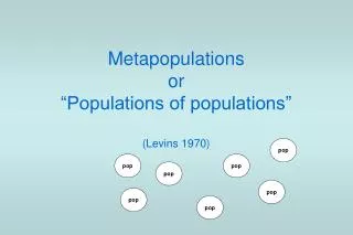
8. Metapopulations N=30 N=30 N=30 N=30 • Metapopulation – A population of populations (Levins, 1970) • How does movement between populations shape the dynamics of extinction and recolonization?

9. A general metapopulation model • Follow the fraction of occupied sites, f • Assume that unoccupied sites are colonized at rate, I • Assume that occupied sites go extinct at rate, E • Then the fraction of occupied sites changes at rate: But what are I and E?

10. A general metapopulation model • Assume that I = pi(1-f) • - Empty patches are colonized at a rate proportional to the product of the probability of local colonization, pi, and the proportion of unoccupied patches, 1-f • Assume that E = pe(f) • - Occupied patches go extinct at a rate proportional to the product of the probability of local extinction, pe, and the proportion of occupied patches, f

11. A general metapopulation model • With these assumptions, we can predict the change in patch occupancy, f • This general model can be used to consider several specific scenarios

12. The mainland-island scenario • Immigrants arrive at a constant rate, pi ,from a mainland source population • Island populations go extinct at a constant rate, pe

13. An example of the mainland-island scenario (The Bay Checkerspot Butterfly) Euphydryas editha Plantago erecta Lives primarily on serpentine soils

14. An example of the mainland-island scenario (The Bay Checkerspot Butterfly) Euphydryas editha

15. The mainland-island scenario • Using these assumptions, we can predict the change in patch occupancy, f • What is the equilibrium proportion of occupied patches for this model?

16. The mainland-island scenario pi = .5 Fraction occupied, f pi = .1 pi = .02 Probability of extinction, pe A small rate of immigration can result in a high proportion of occupied patches. As long as there is some immigration, persistence of the metapopulation is assured!

17. The internal colonization scenario • Immigrants come only from those sites which are currently occupied • As a consequence, pi = i f . • Here i measures how sensitive immigration is to the proportion of occupied patches, f.

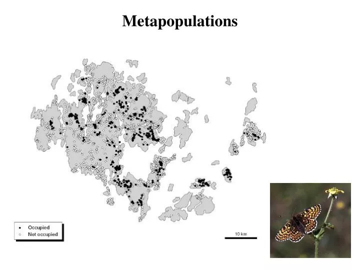
18. An example of internal colonization (The Glanville Fritillary on the Aland Islands) Glanville fritillary (Melitaea cinxia) Plantago lanceolata Veronica spicata

19. An example of internal colonization (The Glanville Fritillary on the Aland Islands) F N S Glanville fritillary (Melitaea cinxia)

20. The internal colonization scenario • Using these assumptions, we can predict the change in patch occupancy, f • What is the equilibrium proportion of occupied patches in this model?

21. The internal colonization scenario Remember: pi = i f  The frequency of immigration increases with increasing i Fraction occupied, f i =.4 i =.2 i =.1 Probability of extinction, pe • Internal colonization is less effective at maintaining the metapopulation than is external colonization. Persistence is not assured. • Nevertheless, internal colonization greatly facilitates metapopulation persistence

22. The rescue effect • To this point we have assumed that the probability of extinction is independent of the fraction of occupied patches • If, however, immigration increases the population size of existing populations, the probability of extinction should decrease as a function of the proportion of occupied patches (e.g., due to decreased demographic stochasticity) 1 e is the maximum extinction probability e pe 0 0 1 f • We can consider this case by setting pe = e(1-f)

23. The rescue effect in the mainland-island scenario • Adding the rescue effect to the mainland-island model: • What is the equilibrium of this model?

24. The rescue effect in the mainland-island scenario pi =.4 pi =.2 Fraction occupied, f pi =.1 All approach pi Maximum probability of extinction, e • The rescue effect facilitates metapopulation persistence • Persistence is assured as long as pi > 0

25. Why do metapopulations matter? (a hypothetical conservation scenario and practice problem) • A 20km2 patch of native prairie exists • A native species of bird occurs exclusively in this native prairie habitat • This species can readily disperse • Only 5km2 can be excluded from development • How should this 5km2 be partitioned?

26. Possibilities for partitioning (a practice problem) Five 1km2 preserves Two 2.5km2 preserves How could we make a scientifically informed decision about which is preferable?

27. Available data for the bird species (a practice problem) • Previous work has shown that the internal colonization rate of this species is: pi = if = .3f • What area do we expect the species to occupy at equilibrium with 2 reserves of size 2.5km2? • What area do we expect the species to occupy at equilibrium with 5 reserves of size 1km2? Probability of extinction (per year) .3 .2 0 2.5 5 1 Patch size (km2)

28. Conclusions from metapopulations • Multiple populations spread the risk of extinction • In some cases, multiple small populations have a larger probability of survival • than few large populations • Dispersal can promote the persistence of metapopulations

29. Exam 3 Results Average: 149 points (75%) # Students Score (in points)