Download
1 / 24
240 likes | 495 Views
Data Structures – LECTURE 2 Elements of complexity analysis. Performance and efficiency Motivation: analysis of Insertion-Sort Asymptotic behavior and growth rates Time and space complexity Big-Oh functions: O(f( n )), Ω( f( n )), Θ( f( n )) Properties of Big-Oh functions.

E N D
Data Structures – LECTURE 2 Elements of complexity analysis • Performance and efficiency • Motivation: analysis of Insertion-Sort • Asymptotic behavior and growth rates • Time and space complexity • Big-Oh functions: O(f(n)), Ω(f(n)), Θ(f(n)) • Properties of Big-Oh functions
Performance and efficiency • We can quantify the performance of a program by measuring its run-time and memory usage. It depends on how fast is the computer, how good the compiler a very local and partial measure! • We can quantify the efficiency of an algorithm by calculating its space and time requirements as a function of the basic units (memory cells and operations) it requires implementation and technology independent!
times n n –1 n –1 n –1 Example of a program analysis Sort the array A of n integers Insertion-Sort(A) • forj 2 toA.length • do keyA[j] • // Insert A[j] into A[1..j-1] • ij – 1 • while i > 0 and A[i] > key • doA[i+1] A[i] • i i – 1 • A[i+1] key cost c1 c2 c4 c5 c6 c7 c8
2 5 4 6 1 3 2 4 5 6 1 3 2 4 5 6 1 3 1 2 4 5 6 3 1 2 3 4 5 6 Insertion-Sort example 5 2 4 6 1 3
Program analysis method • The running time is the sum of the running times of each statement executed • Each statement takes ci steps to execute and is executed ti times total running time is
This is a linear function! Insertion-Sort analysis (1) • Best case: the array is in sorted order, so tj=1 for j=2..n; step 5 takes and steps 6 and 7 are not executed. Thus
This is a quadratic function! Insertion-Sort Analysis (2) • Worst case: the array is in reversed sorted order, so tj=j for j=2..n, so step 5 takes and steps 6 and 7 are always executed, so they take Overall
Asymptotic analysis • We can write the running time of a program T(n) as a function of the input size n: T(n) = f (n) • The function contains constants that are program and platform-dependent. • We are interested in the asymptotic behavior of the program: how quickly does the running time grow as a function of the input size? Rationale: if the input size n is small, all programs are likely to do OK. But they will have trouble when n grows. In fact, the program performance will be dominated by it!
T2(n) = cn2+dn+e T1(n) = an+b overhead n0 No matter what the constants areT2(n) > T1(n)after a while Asymptotic analysis: best vs. worst case for Insertion-Sort time n
To summarize • The efficiency of an algorithm is best characterized by its asymptotic behavior as a function of the input or problem size n. • We are interested in both the run-time and space requirements, as well as the best-case, worst-case, and average behavior of a program. • We can compare algorithms based on their asymptotic behavior and select the one that is best suited for the task at hand.
Time and space complexity • Time complexity: T(n) How many operations are necessary to perform the computation as a function of the input size n. • Space complexity: S(n) How much memory is necessary to perform the computation as a function of the input size n. • Rate of growth: We are interested in how fast the functions T(n) and S(n) grow as a function of the input size n.
Problem size as a function of time • Algorithm Time Maximum problem size • Complexity 1 sec 1 min 1 hour • A1 n 1000 6 x10⁴ 3.6 x 10⁶ • A2 n log2 n 140 4893 2.0 x 10⁵ • A3 n2 31 244 1897 • A4 n3 10 39 153 • A5 2n 9 15 21 Assuming one unit of time equals one millisecond.
Effect of a tenfold speedup • Algorithm Time Maximum problem size • Complexity before speed-up after speed-up • A1 n s1 10s1 • A2 n log2 n s2 approx. 10s2 • (for large s2) • A3 n2 s3 3.16s3 • A4 n3 s4 2.15s4 • A5 2n s5 s5 + 3.3
Asymptotic functions Define mathematical functions that estimate the complexity of algorithm A with a growth rate that is independent of the computer hardware and compiler. The functions ignore the constants and hold for sufficiently large input sizes n. • Upper bound O(f(n)): at most f(n) operations • Lower bound Ω(f(n)): at least f(n) operations • Tight bound Θ(f(n)): order of f(n) operations
cg(n) f(n) n0 f(n) =O(g(n)) Asymptotic upper bound – Big-Oh Let f (n) and g(n) be two functions from naturals to positive reals f (n) = O(g(n)) if there exist c > 0 and n0>1 such that f (n) c×g(n) for all nn0
f(n) cg(n) n0 f(n) = Ω(g(n)) Asymptotic lower bound – Big-Omega Let f (n) and g(n) be two functions from naturals to positive reals f (n) = Ω(g(n)) if there exist c > 0 and n0>1 such that f (n) c×g(n)) for all nn0
c2g(n) f(n) c1g(n) n0 f(n) = Θ(g(n)) Tight bound Asymptotic tight bound – Big-Theta Let f (n) and g(n) be two functions from naturals to positive reals f (n) = Θ(g(n)) if there exist c1,c2 > 0 and n0>1 such that 0 c1×g(n) f (n) c2×g(n) for all nn0
f(n) c2g(n) f(n) cg(n) c1g(n) n0 n0 f(n) = Ω(g(n)) Lower bound f(n) = Θ(g(n)) Tight bound Graphs for O, Ω, and Θ cg(n) f(n) n0 f(n) =O(g(n)) Upper bound
Properties of the O, Ω, and Θ functions Theorem: f is tight iff it is an upper and a lower bound: f (n) = Θ(g(n)) iff f (n) = O(g(n)) and f (n) = Ω(g(n)) • Reflexivity: f (n) = O(f (n)); f (n) = Ω(f (n)); f (n) = Θ(f (n)) • Symmetry: f (n) = Θ(g(n)) iff g(n) = Θ(f (n)) • Transitivity: f(n) = O(g(n)) and g(n) = O(h(n)) then f (n) = O(h(n)) f(n) = Ω(g(n)) and g(n) = Ω(h(n)) then f (n) = Ω(h(n)) f(n) = Θ(g(n)) and g(n) = Θ(h(n)) then f (n) = Θ(h(n))
Properties of the O, Ω, and Θ functions For O, Ω, and Θ: • O(O(f (n)) = O(f (n)) • O(f (n) + g(n)) = O(f (n)) + O(g(n)) • O(f (n).g(n)) = O(f (n)).O(g(n)) • O(log n) = O(lg n) lg is log2 • Polynomials: • Factorials: O(n!) = O(nn+0.5) O(log n!) = O(n lg n)
Asymptotic functions • Asymptotic functions are used in conjunction with recurrence equations to derive complexity bounds • Proving a lower bound for an algorithm is usually harder than proving an upper bound for it. Proving a tight bound is hardest! • Note: still does not answer the if this is the least or the most work for the given problem. For this, we need to consider upper and lower problem bounds (later in the course).