Download
1 / 69
700 likes | 1.12k Views
DATA WAREHOUSE. DATA MINING AND DATA WARE HOUSING. UNIT - I Introduction – Data warehouse delivery method – System Process – Typical process flow within a data warehouse – query management process – process architecture – meta data – data marting. UNIT - II

E N D
DATA MINING AND DATA WARE HOUSING UNIT - I Introduction – Data warehouse delivery method – System Process – Typical process flow within a data warehouse – query management process – process architecture – meta data – data marting. UNIT - II Design aspects – Designing dimension tables – Designing starflake schema – Multi Dimensional Schema – Partition Strategy, Aggregator – Data marting – Meta Data – System Data Warehouse, Process – Load Manager UNIT - III Hardware and operational design – server hardware – network hardware – parallel technology – security input and design of hardware – backup and recovery – service level agreement – operating the hardware
DIMENSIONAL MODELLING • It is the design concept used by many Data Warehouse designers to build their Data Warehouse. • It contains two types of tables • FACT TABLE • DIMENSION TABLE • FACT TABLE • Fact Tables contains the measurements, or metrics or facts of the business process. If your business process is SALES, then the measurement of this business process such as “monthly sales number” is captured into the fact table. In addition to measurements, the only other things a fact table contains are foreign keys for the dimension table
DIMENSION TABLE • Context of measurements are represented in dimension tables. Context of measurement such as who, what, were, when, how of measurement (subject) If your business process is sales (monthly sales no) then measurement can be location (where), time (when), product sold (what) • DIMENSION ATTRIBUTE • This are various columns in a dimension table. In a location dimension, the attributes can be location code, state, country, zip code. • Before designing your DWH, you need to decide what this DWH contains. Ex if you want to build a DWH containing Sales, across multiple locations, across time and across products then your dimensions would • 1) Location 2) Time 3) Product
Each dimension table contains data for one dimension • “ A SCHEMA IS A FACT TABLE PLUS ITS RELATED DIMENSION TABLES”. • Visually, a dimension schema looks very much like a star, hence the term STAR SCHEMA used to describe dimensional model. Fact table reside at the center of the schema, and their dimensions are typically drawn around it.
TIME PRODUCT FACT TABLE (SALES) CLIENT LOCATION
STAR SCHEMA : • A normalized multi-dimensional model in which each disjoint dimension is represented by a single table. • One key principles of dimensional modeling is the use of fully normalized fact tables together with fully de-normalized dimensional tables. • Each dimension table contains data for one dimension. • Why dimensions should be de-normalized ?
In order to query for all locations that are in country ‘USA’. • In OLTP you store location data in multiple tables. • For Ex : 3 Tables
Locations PK Location_id States Countries Loc_name PK State_id PK country_id FK2 State_id State_id country_name FK1 County_id • Now in OLTP the location data may be be spanned across multiple tables. SQL will look like. • SELECT * FROM Location, States, Countries • where locations.state_id = states.state_id • AND Locations.country_id = country.country_id • AND Country_name = ‘USA’ • RELATION IN OLTP
But in OLAP you need to De-Normalized all the data into a single table • Data repeated but makes querying optimized and reduces the query time.
Advantages of the STAR Schema: • Easy for Users to Understand • Optimizes Navigation • Most Suitable for Query Processing • STARjoin and STARindex
Easy for Users to Understand • Users of decision support systems such as data warehouses are different. Here users themselves will formulate queries. When they interact with the data warehouse through third-party query tools, the users should know what to ask for. • They must gain a familiarity with what data is available to them in the data warehouse. • They must have an understanding of the data structures and how the various pieces are associated with one another in the overall scheme. • The STAR schema reflects exactly how the users think and need data for querying and analysis. • When you explain to the users that the units of product A are stored in the fact table and point out the relationship of this piece of data to each dimension table, the user readily understand the connections. • That is because the STAR schema defines the join paths in exactly the same way users normally visualize the relationships.
Optimizes Navigation • In a database schema, what is the purpose of the relationships or connections among the data entities? • A major advantage of the STAR schema is that it optimizes the navigation through the database. • Example: Assume you are the service manager at an automobile dealership selling GM automobiles. You noticed a high incidence of chipped white paint on the Corvettes in January 2000. You need a tool to analyze such defects, determine the underlying causes, and resolve the problems.
TIME (Model year) COMPONENT (Part info) PRODUCT (The make, model, and trim package) DEFECTS (No. Of defects) SUPPLIER (Supplier parts) PROBLEM (Types of problems) Figure: The STAR schema optimizes navigation • Now it is easy to determine the supplier causing the chipped paint on the pearl white corvettes. • Four arrows pointing to the fact table from the four dimension tables show how you will navigate to the rows in the fact table by isolating the Corvette from the product dimension
Most Suitable for Query Processing • Let us form a simple query on the STAR schema for the order analysis. What is the total extended cost of product A sold to customers in San Francisco during January 2000? • First, select the rows from the customer dimension table where the city is San Francisco. Then, from the fact table, select only those rows that are related to these customer dimension rows. This is first set of rows from the fact tables. • Next, select the rows in the Time dimension table where the month is January 2000. Select from the first result set of fact table rows. • Move on to the next dimension of product. Select the rows in the product dimension table where the product is product A • Select from the second result only those rows that are related to the selected product dimension rows.
STARjoin and STARindex • The STAR schema allows the query processor software to use better execution plans. • STARjoin can join more than two tables in a single operation. • STARindex is a specialized index to accelerate joins performance. These are indexes created on one or more foreign keys of the fact table.
SNOW FLAKE SCHEMA : • A normalized multidimensional model in which each disjoint dimension is represented by one or more hierarchical tables FACT SNOWFLAKE STAR DIMENSIONS
FACT SNOWFLAKE STAR DIMENSIONS LOCATIONS DEPARTM BUSINESS UNIT SALES TRANSACTIONS PRODUCTS STYLE LOCATIONS REGION COLOR PRODUCT TIME TIME SIZE WEEK SUMMER SALES EASTER SALES MONTH
Advantages • Small saving in storage space • Normalized structure are easier to update and maintain. Disadvantages • Schema less intuitive and end-users are put off by the complexity. • Ability to browse through the contents difficult. • Degraded query performance because of additional joins.
Fact constellation: Sophisticated applications may require multiple fact tables to share dimension tables. This kind of schema can be viewed as a collection of stars, and hence is called a galaxy schema or a fact constellation. Multiple fact tables that share many dimension tables Booking and Checkout may share many dimension tables in the hotel industry
Examples for Defining Star, Snowflake, and Fact Constellation Schemas Data warehouses and data marts can be defined using two language primitives, one for cube definition and one for dimension definition. $The cube definition statement has the following syntax: define cube <cube name> [<dimension list>]: <measure list> $The dimension definition statement has the following syntax: define dimension <dimension name> as (<attribute or dimension list>) > Star schema definition. DMQL for the above diagram: define cube sales star [time, item, branch, location]: dollars sold = sum(sales in dollars), units sold = count(*) define dimension time as (time key, day, day of week, month, quarter, year)
define dimension item as (item key, item name, brand, type, supplier type) define dimension branch as (branch key, branch name, branch type) define dimension location as (location key, street, city, province or state, country) > Snowflake schema definition. DMQL for the above diagram define cube sales snowflake [time, item, branch, location]: dollars sold = sum(sales in dollars), units sold = count(*) define dimension time as (time key, day, day of week, month, quarter, year) define dimension item as (item key, item name, brand, type, supplier (supplier key, supplier type)) define dimension branch as (branch key, branch name, branch type) define dimension location as (location key, street, city (city key, city, province or state, country))
> Fact constellation schema def. DMQL for the above diagram define cube sales [time, item, branch, location]: dollars sold = sum(sales in dollars), units sold = count(*) define dimension time as (time key, day, day of week, month, quarter, year) define dimension item as (item key, item name, brand, type, supplier type) define dimension branch as (branch key, branch name, branch type) define dimension location as (location key, street, city, province or state, country) define cube shipping [time, item, shipper, from location, to location]: dollars cost = sum(cost in dollars), units shipped = count(*) define dimension time as time in cube sales define dimension item as item in cube sales define dimension shipper as (shipper key, shipper name, location as location in cube sales, shipper type) define dimension from location as location in cube sales define dimension to location as location in cube sales
Measures: Their Categorization and Computation • Distributive • if the result derived by applying the function to n aggregate values is the same as that derived by applying the function on all the data without partitioning. • E.g., count(), sum(), min(), max() • Algebraic • if it can be computed by an algebraic function with M arguments (where M is a bounded integer), each of which is obtained by applying a distributive aggregate function. • E.g., avg(), min_N(), standard_deviation() • Holistic • if there is no constant bound on the storage size needed to describe a sub aggregate. • E.g., median(), mode(), rank()
Concept Hierarchies • A concept hierarchy defines a sequence of mappings from a set of low-level concepts to higher-level, more general concepts. • Many concept hierarchies are implicit within the database schema. • A concept hierarchy that is a total or partial order among attributes in a database schema is called a schema hierarchy. • Specification of hierarchies • Schema hierarchy • day < {month < quarter; week} < year • Set_grouping hierarchy • {1..10} < inexpensive
Concept hierarchies that are common to many applications may be predefined in the data mining system, such as the concept hierarchy for time. • Data mining systems should provide users with the flexibility to tailor predefined hierarchies according to their particular needs. • Concept hierarchies may also be defined by discretizing or grouping values for a given dimension or attribute, resulting in a set-grouping hierarchy. • There may be more than one concept hierarchy for a given attribute or dimension, based on different user viewpoints. • Concept hierarchies may be provided manually by system users, domain experts, or knowledge engineers, or may be automatically generated based on statistical analysis of the data distribution. • Concept hierarchies allow data to be handled at varying levels of abstraction.
Figure : Hierarchical and lattice structures of attributes in warehouse dimensions: (a) a hierarchy for location;(b) a lattice for time.
A Multidimensional Data Model Data warehouses and OLAP tools are based on a multidimensional data model. This model views data in the form of a data cube. From Tables and Spreadsheets to Data Cubes “What is a data cube?” A data cube allows data to be modeled and viewed in multiple dimensions. It is defined by dimensions and facts. A 2-D view of sales data for XYZ according to the dimensions time and item, where the sales are from branches located in the city of Hyderabad.
A 3-D view of sales data for XYZ according to the dimensions time, item and location. A 3-D data cube representation of the data in above Table, according to the dimensions time, item, and location.
Date 2Qtr 1Qtr sum 3Qtr 4Qtr TV Product U.S.A PC VCR sum Canada Country Mexico sum All, All, All A Sample Data Cube Total annual sales of TV in U.S.A.
Cuboids Corresponding to the Cube all 0-D(apex) cuboid country product date 1-D cuboids product,date product,country date, country 2-D cuboids 3-D(base) cuboid product, date, country
Browsing a Data Cube • Visualization • OLAP capabilities • Interactive manipulation
Multidimensional Schemas • Class of decision support queries, that analyze data by representing facts and dimensions within a multidimensional cube. Effects as each dimension will occupy an axis and values within cubes corresponds to factual transformations. • It is used to view the cubes, pivot point, slice and dice. • Ex : Retail Sales Analysis using a cubical representation of products by store by day in a 3-D cube with 3 axes representing Product, Store & Day Time Location Product
Some operations in the multidimensional data model • Roll-up(drill-up)-Performs aggregation on a data cube, either by climbing up a concept hierarchy for a dimension or by dimension reduction. • Drill-down- Reverse of roll-up operation. It navigates from less details data to more detailed data. • Slice- Performs a selection on one dimension of the given cube, resulting in a sub-cube. • Dice- Define a sub-cube by performing a selection on two or more dimensions. • Pivot(rotate)- is a visualization operation that rotates the data axes in a view ,in order to provide an alternative presentation of data.
605 Toronto Vancover Dice for (location=”Toronto “ or “vancover”) and (time=”Q1” or “Q2”) and (item=”H.E” or “comp) Q1 Q2 825 H.E. comp Items (types) Location(Cities) Chicago H.E Comp Phone Security 440 14 NY 605 825 14 400 156 Toronto 395 Vancover 605 825 14 400 Q1 Q2 Q3 Q4 400 Time (quarters) Chicago NY Toronto Vancover Pivot Home comp phone security entertainment Items (types) Chicago slice for time “Q1” NY Toronto Vancover Home comp phone security entertainment
Drill-down ontime(from quarters to months) Chicago Location(Cities) NY Chicago Toronto 440 NY 605 825 14 400 Vancover 156 Toronto Jan 395 Roll-up On location (from cities to country) Vancover Feb Q1 Q2 Q3 Q4 Mar App Time (quarters) May June July Home comp phone security entertainment USA August Canada Time (months) Items (types) Q1 Q2 Q3 Q4 Sep Oct Nov Dec H.E comp phone security Items (types) H.E comp phone security Items (types)
Product by store by day cube • The point of intersection of all axes represents the actual number of sales for a specific product, in a specific store, on a specific day. • Also alternatively if we wish to view sum of all sales by a specific store and a specific day. • Aggregation function would be applied by slice and dice Sum of all (Products) Location Sum (Products)
DataWarehouse Architecture • Steps for the Design and Construction of DataWarehouses : • A) Business Analysis Framework • Four different views regarding the design of a data warehouse must be considered: the top-down view, the data source view, the data warehouse view, and the business query view • . • The top-down view allows the selection of the relevant information necessary for the data warehouse. This information matches the current and future business needs. • The data source view exposes the information being captured, stored, and managed by operational systems. This information may be documented at various levels of detail and accuracy, from individual data source tables to integrated data source tables. Data sources are often modeled by traditional data modeling techniques, such as the entity-relationship model or CASE (computer-aided • software engineering) tools.
The data warehouse view includes fact tables and dimension tables. It represents the information that is stored inside the data warehouse, including precalculated totals and counts, as well as information regarding the source, date, and time of origin, added to provide historical context. Finally, the business query view is the perspective of data in the data warehouse from the viewpoint of the end user.
B) The Process of Data Warehouse Design • In general, the warehouse design process consists of the following steps: • 1. Choose a business process to model, for example, orders, invoices, shipments, inventory, account administration, sales, or the general ledger. If the business process is organizational and involves multiple complex object collections, a data warehouse model should be followed. However, if the process is departmental and focuses on the analysis of one kind of business process, a data mart model should be chosen. • 2. Choose the grain of the business process. The grain is the fundamental, atomic level of data to be represented in the fact table for this process, for example, individual transactions, individual daily snapshots, and so on.
3. Choose the dimensions that will apply to each fact table record. Typical dimensions are time, item, customer, supplier, warehouse, transaction type, and status. 4. Choose the measures that will populate each fact table record. Typical measures are numeric additive quantities like dollars sold and units sold.
1. The bottom tier is a warehouse database server that is almost always a relational database system. Back-end tools and utilities are used to feed data into the bottom tier from operational databases or other external sources 2. The middle tier is an OLAP server that is typically implemented using either (1) a relational OLAP (ROLAP) model, that is, an extended relational DBMS that maps operations on multidimensional data to standard relational operations; or (2) a multidimensional OLAP (MOLAP) model, that is, a special-purpose server that directly implements multidimensional data and operations. 3.The top tier is a front-end client layer, which contains query and reporting tools, analysis tools, and/or data mining tools (e.g., trend analysis, prediction, and so on).
Enterprise warehouse: An enterprise warehouse collects all of the information about subjects spanning the entire organization. Data mart: A data mart contains a subset of corporate-wide data that is of value to a specific group of users. Virtual warehouse: A virtual warehouse is a set of views over operational databases.
3. DataWarehouse Back-End Tools and Utilities Data warehouse systems use back-end tools and utilities to populate and refresh their data. These tools and utilities include the following functions: Data extraction,which typically gathers data frommultiple, heterogeneous, and external sources Data cleaning, which detects errors in the data and rectifies them when possible Data transformation, which converts data from legacy or host format to warehouse format. Load, which sorts, summarizes, consolidates, computes views, checks integrity, builds indices and partitions Refresh, which propagates the updates from the data sources to the warehouse
Metadata Repository Metadata are data about data.When used in a data warehouse, metadata are the data that define warehouse objects. Additional metadata are created and captured for timestamping any extracted data, the source of the extracted data, and missing fields that have been added by data cleaning or integration processes. A metadata repository should contain the following: 1) A description of the structure of the data warehouse, which includes the warehouse schema, view, dimensions, hierarchies, and derived data definitions, as well as data mart locations and contents 2) Operational metadata, which include data lineage (history of migrated data and the sequence of transformations applied to it), currency of data (active, archived, or purged), and monitoring information (warehouse usage statistics, error reports, and audit trails)
3) The algorithms used for summarization, which include measure and dimension definition algorithms, data on granularity, partitions, subject areas, aggregation, summarization, and predefined queries and reports 4) The mapping from the operational environment to the data warehouse, which includes source databases and their contents, gateway descriptions, data partitions, data extraction, cleaning, transformation rules and defaults, data refresh and purging rules, and security (user authorization and access control) 5) Data related to system performance, which include indices and profiles that improve data access and retrieval performance, in addition to rules for the timing and scheduling of refresh, update, and replication cycles 6) Business metadata, which include business terms and definitions, data ownership information, and charging policies