Download
1 / 38
450 likes | 693 Views
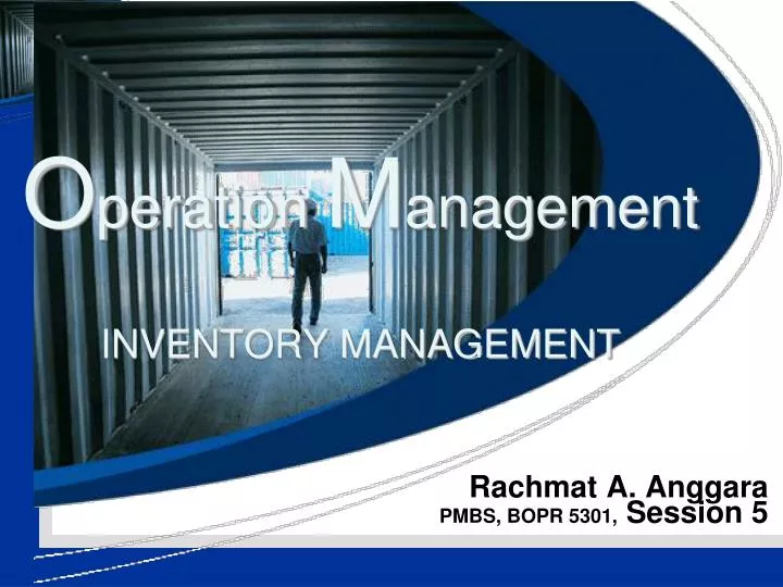
O peration M anagement INVENTORY MANAGEMENT. Rachmat A. Anggara PMBS, BOPR 5301, Session 5. INVENTORY??. INVENTORY is…. One of the most expensive assets of many companies representing as much as 50% of total invested capital

E N D
Operation ManagementINVENTORY MANAGEMENT Rachmat A. Anggara PMBS, BOPR 5301, Session 5
INVENTORY is… • One of the most expensive assets of many companies representing as much as 50% of total invested capital • Operations managers must balance inventory investment and customer service
Type of INVENTORY … • Raw material • Purchased but not processed • Work-in-process • Undergone some change but not completed • A function of cycle time for a product • Maintenance/repair/operating (MRO) • Necessary to keep machinery and processes productive • Finished goods • Completed product awaiting shipment
Cycle time 95% 5% Input Wait for Wait to Move Wait in queue Setup Run Output inspection be moved time for operator time time Material Flow Cycle..
INVENTORY Management.. • How inventory items can be classified • How accurate inventory records can be maintained • How inventory cost can be minimized while keep customer order fulfilled
INVENTORY Management.. • Record Accuracy. • Manual. • Automate. • Cycle Counting. • Reconciliation of inventory. • ABC analysis system. • Control of Service Inventories. • Good personnel selection, training, and discipline • Tight control on incoming shipments • Effective control on all goods leaving facility
#12572 600 $ 14.17 $ 8,502 3.7% C #14075 2,000 .60 1,200 .5% C #01036 50% 100 8.50 850 .4% 5% C #01307 1,200 .42 504 .2% C #10572 250 .60 150 .1% C ABC-Analysis Item Stock Number Percent of Number of Items Stocked Annual Volume (units) x Unit Cost = Annual Dollar Volume Percent of Annual Dollar Volume Class #10286 20% 1,000 $ 90.00 $ 90,000 38.8% 72% A 17.5 % #11526 500 154.00 77,000 33.2% A 1,550 17.00 26,350 11.3% B #12760 30% 23% 33.9 % #10867 350 42.86 15,001 6.4% B #10500 1,000 12.50 12,500 5.4% B 48.5 %
A Items 80 – 70 – 60 – 50 – 40 – 30 – 20 – 10 – 0 – Percent of annual dollar usage B Items C Items | | | | | | | | | | 10 20 30 40 50 60 70 80 90 100 Percent of inventory items ABC-Analysis Pareto rule..
Control of Inventory • Can be a critical component of profitability • Losses may come from shrinkage or pilferage • Applicable techniques include • Good personnel selection, training, and discipline • Tight control on incoming shipments • Effective control on all goods leaving facility
Average inventory on hand Q 2 Usage rate Inventory level Minimum inventory Time 1. Economic Order Quantity Inventory Usage overtime Order quantity = Q (maximum inventory level)
Curve for total cost of holding and setup Minimum total cost Holding cost curve Annual cost Setup (or order) cost curve Order quantity Optimal order quantity 1. Economic Order Quantity Objective Minimise Cost Table 11.5
Annual demand Number of units in each order Setup or order cost per order = = (S) D Q 1. Economic Order Quantity CalculateSetup Cost Q = Number of pieces per order Q* = Optimal number of pieces per order (EOQ) D = Annual demand in units for the Inventory item S = Setup or ordering cost for each order H = Holding or carrying cost per unit per year Annual setup cost = (Number of orders placed per year) x (Setup or order cost per order)
Order quantity 2 = (Holding cost per unit per year) = (H) Q 2 1. Economic Order Quantity CalculateHolding Cost Q = Number of pieces per order Q* = Optimal number of pieces per order (EOQ) D = Annual demand in units for the Inventory item S = Setup or ordering cost for each order H = Holding or carrying cost per unit per year Annual holding cost = (Average inventory level) x (Holding cost per unit per year)
D Q Annual setup cost = S Annual holding cost = H Q 2 D Q S = H 2DS = Q2H Q2 = 2DS/H Q* = 2DS/H Q 2 1. Economic Order Quantity Optimal order quantity is found when annual setup cost equals annual holding cost Solving for Q*
2DS H Q* = 2(1,000)(10) 0.50 Q* = = 40,000 = 200 units 1. Economic Order Quantity(Example) Determine optimal number of needles to order D = 1,000 units S = $10 per order H = $.50 per unit per year
Expected number of orders Demand Order quantity D Q* = N = = 1,000 200 N = = 5 orders per year 1. Economic Order Quantity(Example) Determine optimal number of needles to order D = 1,000 units Q* = 200 units S = $10 per order H = $.50 per unit per year
Q 2 D Q 200 2 TC = S + H 1,000 200 TC = ($10) + ($.50) 1. Economic Order Quantity(Example) Determine optimal number of needles to order D = 1,000 units Q* = 200 units S = $10 per order N = 5 orders per year H = $.50 per unit per year T = 50 days Total annual cost = Setup cost + Holding cost TC = (5)($10) + (100)($.50) = $50 + $50 = $100
Lead time for a new order in days ROP = Demand per day D Number of working days in a year d = 1. Economic Order Quantity(Reorder Point) • EOQ answers the “how much” question • The reorder point (ROP) tells when to order = d x L
D Number of working days in a year d = 1. Economic Order Quantity(Reorder Point) Demand = 8,000 DVDs per year 250 working day year Lead time for orders is 3 working days = 8,000/250 = 32 units ROP = d x L = 32 units per day x 3 days = 96 units
2. Production Order Quantity • Used when inventory builds up over a period of time after an order is placed • Used when units are produced and sold simultaneously
Part of inventory cycle during which production (and usage) is taking place Demand part of cycle with no production Inventory level Maximum inventory t Time 2. Production Order Quantity
= (Average inventory level) x Annual inventory holding cost Annual inventory level Holding cost per unit per year = (Maximum inventory level)/2 Maximum inventory level Total produced during the production run Total used during the production run = – = pt – dt 2. Production Order Quantity Q = Number of pieces per order p = Daily production rate H = Holding cost per unit per year d = Daily demand/usage rate t = Length of the production run in days
Q2 = 2DS H[1 - (d/p)] 2DS H[1 - (d/p)] Q* = 2. Production Order Quantity Q = Number of pieces per order p = Daily production rate H = Holding cost per unit per year d = Daily demand/usage rate t = Length of the production run in days Setup cost = (D/Q)S Holding cost = 1/2 HQ[1 - (d/p)] (D/Q)S = 1/2 HQ[1 - (d/p)]
2(1,000)(10) 0.50[1 - (4/8)] Q* = = 80,000 = 282.8 or 283 hubcaps 2DS H[1 - (d/p)] Q* = 2. Production Order Quantity(example) D = 1,000 units p = 8 units per day S = $10 d = 4 units per day H = $0.50 per unit per year
QH 2 D Q TC = S + + PD 3. Quantity Discount Model • Reduced prices are often available when larger quantities are purchased • Trade-off is between reduced product cost and increased holding cost Total cost = Setup cost + Holding cost + Product cost
3. Quantity Discount Model A typical quantity discount schedule
2DS IP Q* = 3. Quantity Discount Model Steps in analyzing a quantity discount For each discount, calculate Q*, I= holding cost, P= percentage If Q* for a discount doesn’t qualify, choose the smallest possible order size to get the discount Compute the total cost for each Q* or adjusted value from Step 2 Select the Q* that gives the lowest total cost
Example 9 2(5,000)(49) (.2)(5.00) 2(5,000)(49) (.2)(4.80) 2(5,000)(49) (.2)(4.75) Q1* = = 700 cars order Q2* = = 714 cars order Q3* = = 718 cars order 3. Quantity Discount Model(example) Calculate Q* for every discount
2(5,000)(49) (.2)(5.00) 2(5,000)(49) (.2)(4.80) 2(5,000)(49) (.2)(4.75) Q1* = = 700 cars order Q2* = = 714 cars order Q3* = = 718 cars order 1,000 — adjusted 2,000 — adjusted 3. Quantity Discount Model(example) Adjusting Q* for every discount
3. Quantity Discount Model(example) Choose the price and quantity that gives the lowest total cost Buy 1,000 units at $4.80 per unit
4. Probabilistic Model • Used when demand is not constant or certain • Use safety stock to achieve a desired service level and avoid stockouts ROP = d x L + ss Annual stockout costs = the sum of the units short x the probability x the stockout cost/unit x the number of orders per year
4. Probabilistic Model ROP = 50 units Stockout cost = $40 per frame Orders per year = 6 Carrying cost = $5 per frame per year
4. Probabilistic Model ROP = 50 units Stockout cost = $40 per frame Orders per year = 6 Carrying cost = $5 per frame per year A safety stock of 20 frames gives the lowest total cost ROP = 50 + 20 = 70 frames
4. Probabilistic Model Safety stock Another method for calculating safety stock.. ROP = demand during lead time + Zsdlt where Z = number of standard deviations sdlt = standard deviation of demand during lead time
4. Probabilistic Model Example… Average demand = m = 350 kits Standard deviation of demand during lead time = sdlt = 10 kits 5%stockout policy (service level = 95%) Using Appendix I, for an area under the curve of 95%, the Z = 1.65 Safety stock = Zsdlt= 1.65(10) = 16.5 kits Reorder point = expected demand during lead time + safety stock = 350 kits + 16.5 kits of safety stock = 366.5 or 367 kits
2DS H 2DS IP Q* = Q* = 2DS H[1 - (d/p)] Q* = Resume of Inventory Model ROP = d x L + ss