Download
1 / 24
480 likes | 1.61k Views
CP302 Separation Process Principles. Mass Transfer - Set 4. CP302 Separation Process Principles. Reference books used for ppts. C.J. Geankoplis Transport Processes and Separation Process Principles 4 th edition, Prentice-Hall India J.D. Seader and E.J. Henley

E N D
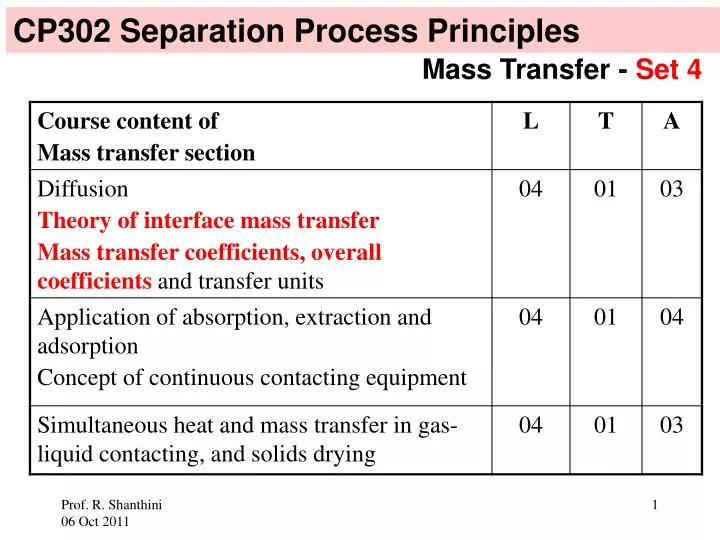
CP302 Separation Process Principles Mass Transfer - Set 4
CP302 Separation Process Principles Reference books used for ppts • C.J. Geankoplis • Transport Processes and Separation Process Principles • 4th edition, Prentice-Hall India • J.D. Seader and E.J. Henley • Separation Process Principles • 2nd edition, John Wiley & Sons, Inc. • 3. J.M. Coulson and J.F. Richardson • Chemical Engineering, Volume 1 • 5th edition, Butterworth-Heinemann
Microscopic (or Fick’s Law) approach: dCA (1) JA = - DAB dz good for diffusion dominated problems Macroscopic (or mass transfer coefficient) approach: ΔCA (50) NA = - k where k is known as the mass transfer coefficient good for convection dominated problems
Mass Transfer Coefficient Approach (CA1 – CA2 ) (51) NA = kc ΔCA = kc kc is the liquid-phase mass-transfer coefficient based on a concentration driving force. CA1 A & B What is the unit of kc? NA CA2
Mass Transfer Coefficient Approach (CA1 – CA2 ) (51) NA = kc ΔCA = kc Using the following relationships between concentrations and partial pressures: CA1 = pA1 / RT; CA2 = pA2 / RT Equation (51) can be written as (pA1 – pA2) / RT (pA1 – pA2) NA = kc = kp (52) (53) where kp = kc / RT kp is a gas-phase mass-transfer coefficient based on a partial-pressure driving force. What is the unit of kp?
Models for mass transfer between phases Mass transfer between phases across the following interfaces are of great interest in separation processes: - gas/liquid interface - liquid/liquid interface Such interfaces are found in the following separation processes: - absorption - distillation - extraction - stripping
Models for mass transfer at a fluid-fluid interface Theoretical models used to describe mass transfer between a fluid and such an interface: - Film Theory - Penetration Theory - Surface-Renewal Theory - Film Penetration Theory
Film Theory Entire resistance to mass transfer in a given turbulent phase is in a thin, stagnant region of that phase at the interface, called a film. Liquid film For the system shown, gas is taken as pure component A, which diffuses into nonvolatile liquid B. pA Bulk liquid CAi In reality, there may be mass transfer resistances in both liquid and gas phases. So we need to add a gas film in which gas is stagnant. Gas CAb z=0 z=δL Mass transport
Two Film Theory There are two stagnant films (on either side of the fluid-fluid interface). Each film presents a resistance to mass transfer. Concentrations in the two fluid at the interface are assumed to be in phase equilibrium. Liquid film Gas film Gas phase Liquid phase pAb pAi CAi CAb Mass transport
Liquid film Gas film Gas phase Liquid phase pAb pAi CAi CAb Mass transport Two Film Theory Interface Interface Gas phase Liquid phase pAb pAi CAi CAb Mass transport Concentration gradients for the film theory More realistic concentration gradients
Two Film Theory applied at steady-state Mass transfer in the gas phase: (pAb – pAi) NA = kp (52) Mass transfer in the liquid phase: Liquid film Gas film NA (CAi – CAb ) (51) = kc Gas phase Liquid phase Phase equilibrium is assumed at the gas-liquid interface. Applying Henry’s law, pAb pAi CAi CAb pAi = HA CAi (53) Mass transport, NA
Henry’s Law pAi = HA CAi at equilibrium, where HA is Henry’s constant for A Note that pAi is the gas phase pressure and CAi is the liquid phase concentration. Liquid film Gas film pAb pAi Unit of H: [Pressure]/[concentration] = [ bar / (kg.m3) ] CAi CAb
Two Film Theory applied at steady-state We know the bulk concentration and partial pressure. We do not know the interface concentration and partial pressure. Liquid film Therefore, we eliminate pAi and CAi from (51), (52) and (53) by combining them appropriately. Gas film Gas phase Liquid phase pAb pAi CAi CAb Mass transport, NA
Two Film Theory applied at steady-state NA From (52): pAi = pAb - (54) kp NA From (51): CAi = CAb + (55) kc Substituting the above in (53) and rearranging: pAb - HACAb NA = (56) HA / kc + 1 / kp The above expression is based on gas-phase and liquid-phase mass transfer coefficients. Let us now introduce overall gas-phase and overall liquid-phase mass transfer coefficients.
Introducing overall gas-phase mass transfer coefficient: Let’s start from (56). Introduce the following imaginary gas-phase partial pressure: pA*≡ HACAb (57) where pA*is a partial pressure that would have been in equilibrium with the concentration of A in the bulk liquid. Introduce an overall gas-phase mass-transfer coefficient (KG) as 1 1 HA ≡ + (58) KG kp kc Combining (56), (57) and (58): NA = KG (pAb- pA*) (59)
Introducing overall liquid-phase mass transfer coefficient: Once again, let’s start from (56). Introduce the following imaginary liquid-phase concentration: pAb≡ HACA* (60) where CA*is a concentration that would have been in equilibrium with the partial pressure of A in the bulk gas. Introduce an overall liquid-phase mass-transfer coefficient (KL) as 1 1 1 ≡ + (61) KL HAkp kc Combining (56), (60) and (61): NA = KL (CA*- CAb) (62)
Gas-Liquid Equilibrium Partitioning Curve showing the locations of p*A and C*A pA pAb pAb = HACA* pAi pAi = HA CAi pA* pA* = HA CAb CAb CAi CA* CA
Summary: NA = KL (CA*- CAb) (62) = KG (pAb- pA*) (59) where CA*= pAb/ HA (60) pA*= HACAb (57) 1 HA 1 HA = = + (58 and 61) KG KL kp kc
Example 3.20 from Ref. 2 (modified) Sulfur dioxide (A) is absorbed into water in a packed column. At a certain location, the bulk conditions are 50oC, 2 atm, yAb = 0.085, and xAb = 0.001. Equilibrium data for SO2 between air and water at 50oC are the following: Experimental values of the mass transfer coefficients are kc= 0.18 m/h and kp = 0.040 kmol/h.m2.kPa. Compute the mass-transfer flux by assuming an average Henry’s law constant and a negligible bulk flow.
Solution: Data provided: T = 273oC + 50oC = 323 K; PT = 2 atm; yAb = 0.085; xAb = 0.001; kc= 0.18 m/h; kp = 0.040 kmol/h.m2.kPa HA = 1.4652 atm.m3/kmol slope of the curve HA = 161.61 kPa.m3/kmol
Equations to be used: NA = KL (CA*- CAb) (62) = KG (pAb- pA*) (59) where CA*= pAb/ HA (60) pA*= HACAb (57) 1 HA 1 HA = = + (58 and 61) KG KL kp kc
Calculation of overall mass transfer coefficients: 1 HA 1 HA = = + (58 and 61) KG KL kp kc 1 1 = h.m2.kPa/kmol = 25 h.m2.kPa/kmol kp 0.040 HA 161.61 kPa.m3/kmol = = 897 h.m2.kPa/kmol kc 0.18 m/h KG = 1/(25 + 897) = 1/922 = 0.001085 kmol/h.m2.kPa KL = HAKG = 161.61/922 = 0.175 m/h
NA = KL (CA*- CAb) (62) is used to calculate NA CA*= pAb/ HA = yAbPT / HA = 0.085 x 2 atm / 1.4652 atm.m3/kmol = 0.1160 kmol/m3 CAb= xAbCT = 0.001 CT CT = concentration of water (assumed) = 1000 kg/m3 = 1000/18 kmol/m3 = 55.56 kmol/m3 CAb= 0.001 x 55.56 kmol/m3 = 0.05556 kmol/m3 NA = (0.175 m/h)(0.1160 - 0.05556) kmol/m3 = 0.01058 kmol/m2.h
Alternatively, NA = KG (pAb - pA*) (59) is used to calculate NA pA*= CAbHA = xAbCTHA = 0.001 x 55.56 x 161.61 kPa = 8.978 kPa pAb= yAbPT = 0.085 x 2 x 1.013 x 100 kPa = 17.221 kPa NA = (1/922 h.m2.kPa/kmol)(17.221 - 8.978) kPa = 0.00894 kmol/m2.h


![[PDF READ ONLINE] Transport Processes and Separation Process Principles (Include](https://cdn7.slideserve.com/12653951/pdf-read-online-transport-processes-dt.jpg)