Download
1 / 25
250 likes | 372 Views
Spatially Assessing Model Error Using Geographically Weighted Regression. Shawn Laffan Geography Dept ANU. Non-spatial methods are increasingly used to model and map continuous spatial properties Artificial Neural Networks, Decision Trees, Expert Systems...

E N D
Spatially Assessing Model Error Using Geographically Weighted Regression Shawn Laffan Geography Dept ANU
Non-spatial methods are increasingly used to model and map continuous spatial properties • Artificial Neural Networks, Decision Trees, Expert Systems... • These can use more ancillary variables than explicitly spatial methods • Usually assessed using non-spatial global error measures • Summarise many data points • Cannot easily identify where model is correct
Error residuals may be mapped • But usually points • Difficult to visually identify spatial clustering • Large point symbols • no multi-scale • no quantification • Can use spatial error analysis to detect clusters of similar prediction • Use these areas with confidence • Areas with unacceptable error indicate need for different variables or approach
To spatially assess model error a method should: • Locally calculate omission, commission & total error in original data units in one assessment • one dataset each • Assess error for unsampled locations • generate spatially continuous surfaces for easier interpretation • Provide confidence information about the assessment • uncertainty estimate
Possible approaches: • Mean, StdDev, Range for spatial window • three attributes to interpret for each of omission, commission and total error • mean will often not equal zero • Co-variograms • global assessment • work only for sampled locations • Local Spatial Autocorrelation • Geographically Weighted Regression
Local Spatial Autocorrelation: • indices of spatial association • easy to interpret • multi-scale • calculate residuals and assess spatial clustering • some indices calculable for unsampled locations • Getis-Ord Gi*, Openshaw’s GAM
Local Spatial Autocorrelation: • Give difference from expected (global mean) • mean will not normally be zero • Must analyse omission & commission separately • partly cancel out • leads to numeric and sample density problems • confidence information
Geographically Weighted Regression • multivariate spatial analysis in the presence of non-stationarity • perform regression within a moving spatial window • multi-scaled • can directly assess residual error without prior calculation • simultaneous omission, commission and total error assessment • estimates for unsampled locations • r2 parameter gives confidence information
The approach: • Ordinary Least Squares • Y = a + bX • calculated for circles of increasing radius across the entire dataset • minimum 5 sample points • no spatial weight decay with distance • does not force an assumed distribution on the data • optimal spatial scale when r2 is maximum
Interpreting regression parameters for error: • error is the square root of the area between the fitted and the optimal lines • this is bounded by the min and max of the predicted distribution • as b approaches 1 the intercept approaches +/- infinity causing extremely large error values • use the intersection of the fitted line with the optimal line (1:1, Y=X) to determine omission & commission
The r2 parameter • high r2 means reliable b parameters and therefore reliable error measures • low values indicate low confidence caused by dispersed data values • these areas cannot be used as b is meaningless
Example application • feed-forward ANN to infer aluminium oxide • used topographic and vegetation indices • 1100 km2 area at Weipa, Far North Queensland, Australia • 16000 drill cores • 30.4% accurate within +/- 1 original unit • 48.7% accurate within +/- 2 original units
Omission Commission Total
Optimal spatial lag Max r2
Visualising error distribution with confidence information r2 = red omission = green commission = blue
Limitations • sample density & distribution • outliers • data & spatial • cause low r2 • landscape does not operate in circles
Extended Utility • can use the regression parameters to correct the ANN prediction • similar to universal kriging but ANN allows for the inclusion of more ancillary variables • have not taken into account r2 values
Conclusions: • GWR allows the spatial investigation of non-spatial model error • calculates total, omission and commission error in one assessment, with confidence information • identified locations of good and poor model prediction in a densely sampled dataset • not immediately obvious without GWR • currently exploratory • significance tests would be useful