Download
1 / 33
330 likes | 537 Views
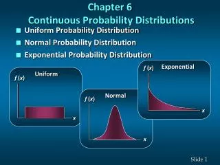
Chapter 6 Continuous Probability Distributions. Normal Probability Distribution. f ( x ). x. . Continuous Probability Distributions. A continuous random variable can assume any value in an interval on the real line or in a collection of intervals.

E N D
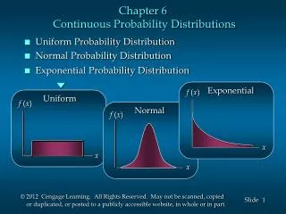
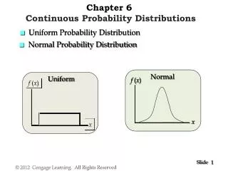
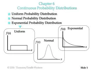
Chapter 6 Continuous Probability Distributions • Normal Probability Distribution f(x) x
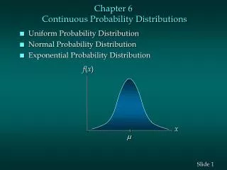
Continuous Probability Distributions • A continuous random variable can assume any value in an interval on the real line or in a collection of intervals. • It is not possible to talk about the probability of the random variable assuming a particular value. • Instead, we talk about the probability of the random variable assuming a value within a given interval. • The probability of the random variable assuming a value within some given interval from x1 to x2 is defined to be the area under the graph of the probability density function between x1and x2.
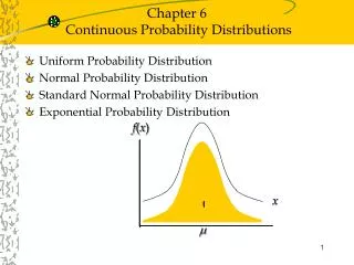
Normal Probability Distribution • The normal probability distribution is the most important distribution for describing a continuous random variable. • It has been used in a wide variety of applications: • Heights and weights of people • Test scores • Scientific measurements • Amounts of rainfall • It is widely used in statistical inference
Normal Probability Distribution • Normal Probability Density Function where: = mean = standard deviation = 3.14159 e = 2.71828
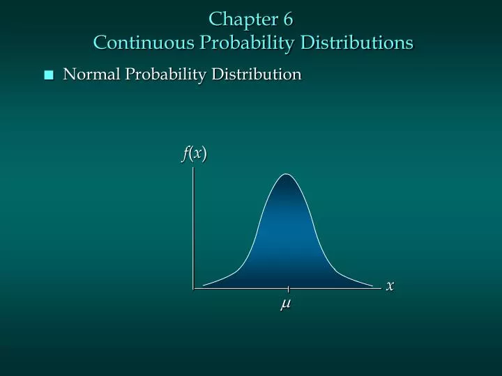
Normal Probability Distribution • Graph of the Normal Probability Density Function f(x) x
Normal Probability Distribution • Characteristics of the Normal Probability Distribution • The distribution is symmetric, and is often illustrated as a bell-shaped curve. • Two parameters, m (mean) and s (standard deviation), determine the location and shape of the distribution. • The highest point on the normal curve is at the mean, which is also the median and mode. • The mean can be any numerical value: negative, zero, or positive. … continued
Normal Probability Distribution • Characteristics of the Normal Probability Distribution • The standard deviation determines the width of the curve: larger values result in wider, flatter curves. s = 10 s = 50
Normal Probability Distribution • Characteristics of the Normal Probability Distribution • The total area under the curve is 1 (.5 to the left of the mean and .5 to the right). • Probabilities for the normal random variable are given by areas under the curve.
The standard normal curve is symmetric about its mean (μ=0) and has a total area of one under it and above the z axis. point of inflection 0 Z
Find the area under the standard normal distribution for z values between z = 0 and z = 2.53. [Or P(0<z<2.53)=?] .4943 0 2.53 Z
Find P(z>-1.14). -1.14 0
P(z>-1.14)=.3729+.5000 =.8729 .3729 .5000 -1.14 0
Find P(-1.28<z<1.83). -1.28 0 1.83 Z
P(-1.28<z<1.83)=.3997+.4664 =.8661 .4664 .3997 -1.28 1.83
Find P(-2.54<z<-.42). -2.54 -.42
P(-2.54<z<-.42) =.4945-.1628 =.3317 Dark blue shaded area is .1628=P(0<z<.42). Total shaded area is .4945=P(0<z<2.54). -2.54 -.42
Find c so that P(0<z<c) = .4772. Find c so that the shaded area is .4772. 0 z=c Z
P(0<z<2.0)=.4772 0 z=2.0 Z
Normal Probability Distribution • Characteristics of the Normal Probability Distribution • 68.26% of values of a normal random variable are within +/- 1standard deviation of its mean. • 95.44% of values of a normal random variable are within +/- 2standard deviations of its mean. • 99.72% of values of a normal random variable are within +/- 3standard deviations of its mean.
Standard Normal Probability Distribution • A random variable that has a normal distribution with a mean of zero and a standard deviation of one is said to have a standard normal probability distribution. • The letter z is commonly used to designate this normal random variable. • Converting to the Standard Normal Distribution • We can think of z as a measure of the number of standard deviations x is from .
What if we have a normal population with mean of 50 and a standard deviation of 5. That is 50 X
If we have a normal population with mean of 50 and a standard deviation of 5. We can standardize the scores by finding their corresponding z-scores. That is 50 X 0 Z
If we have a normal population with mean of 50 and a standard deviation of 5. What is the probability that a randomly selected element of the population will have a value larger than 58? 50 58 X We must first find a z-score for x = 58.
P(0<z<1.6)=.4452 0 1.6 Z P(z>1.6)=.0548
Example: Pep Zone • Standard Normal Probability Distribution Pep Zone sells auto parts and supplies including a popular multi-grade motor oil. When the stock of this oil drops to 20 gallons, a replenishment order is placed. The store manager is concerned that sales are being lost due to stockouts while waiting for an order. It has been determined that leadtime demand is normally distributed with a mean of 15 gallons and a standard deviation of 6 gallons. The manager would like to know the probability of a stockout, P(x > 20).
Area = .2967 Area = .5 - .2967 = .2033 Area = .5 z 0 .83 Example: Pep Zone • Standard Normal Probability Distribution The Standard Normal table shows an area of .2967 for the region between the z = 0 and z = .83 lines below. The shaded tail area is .5 - .2967 = .2033. The probability of a stock- out is .2033. z = (x - )/ = (20 - 15)/6 = .83
Example: Pep Zone • Using the Standard Normal Probability Table
Example: Pep Zone • Standard Normal Probability Distribution If the manager of Pep Zone wants the probability of a stockout to be no more than .05, what should the reorder point be? Let z.05 represent the z value cutting the .05 tail area. Area = .05 Area = .5 Area = .45 z.05 0
Example: Pep Zone • Using the Standard Normal Probability Table We now look-up the .4500 area in the Standard Normal Probability table to find the corresponding z.05 value. z.05 = 1.645 is a reasonable estimate.
Example: Pep Zone • Standard Normal Probability Distribution The corresponding value of x is given by x = + z.05 = 15 + 1.645(6) = 24.87 A reorder point of 24.87 gallons will place the probability of a stockout during leadtime at .05. Perhaps Pep Zone should set the reorder point at 25 gallons to keep the probability under .05.
Applications Where the Area Under a Normal Curve is Provided Let X be a normal random variable describing life of a certain brand of light bulbs with mean of 500 hours and standard deviation of 65 hours. Find the time that at least 75% of the light bulbs will last longer than.
First find a z so that 75% of the area under the normal curve lies to the right of z. .2500 .5000 z = -.67
Now convert this z score to hours of life for the light bulbs. 75% of the light bulbs should last longer than 456.45 hours