Download
1 / 27
280 likes | 390 Views
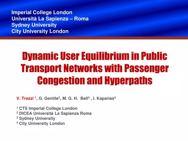
Imperial College London Università La Sapienza – Roma Sydney University City University London. Dynamic User Equilibrium in Public Transport Networks with Passenger Congestion and Hyperpaths. V. Trozzi 1 , G. Gentile 2 , M. G. H. Bell 3 , I. Kaparias 4

E N D
Imperial College London Università La Sapienza – Roma Sydney University City University London Dynamic User Equilibrium in Public Transport Networks with Passenger Congestion and Hyperpaths V. Trozzi 1, G. Gentile2, M. G. H. Bell3, I. Kaparias4 1 CTS Imperial College London2 DICEA Università La Sapienza Roma3Sydney University 4City University London
Hyperpath : what is this?Strategy on Transit Network d o 2 BUS STOP 1 1 1 BUS STOP 2 2 1 1 3 BUS STOP 3 3 3 4 3 4
Hyperpaths : why?Rational choice - Waiting - Variance + Riding + Walking = + Utility d o 2 BUS STOP 1 1 1 BUS STOP 2 2 1 1 3 BUS STOP 3 3 3 4 3 4
Dynamic Hyperpaths:queues of passengers at stops – capacity constraits d o 2 BUS STOP 1 1 1 BUS STOP 2 2 1 1 3 BUS STOP 3 3 3 4 3 4
Dynamic User Equilibrium model : fixed point problem dynamic temporal profiles Uncongested Network Assignment Map per destination cost ArcPerformance Functions
4. Arc Performance Functions The APF of each arc aAdetermines the temporal profile of exit time for any arc, given the entry time .
4. Arc Performance Functions Bottleneck queue model Phase 2: (uncongested) Waiting Phase 1: Queuing Phase 2: Waiting Phase 1: Queuing
4. Arc Performance Functions propagation of available capacity Available capacity τ b dwelling riding a’’ waiting queuing • a’
4. Arc Performance Functions bottleneck queue model Time varying bottleneck FIFO The above Qout is different from that resulting from network propagation: this is not a DNL they are the same only at the fixed point
4. Arc Performance Functionsnumbur of arrivals to wait before boarding While queuing some busses pass at the stop
Hypergraph and Model Graph LAa LAa WAa a QAa
1. Stop model 2 2 h = a1a2 1 Line nodes Stop node 1 a2 23 2 a1 BUS STOP 1 1 2 1 23 23 h = a2a23 a2 1 1 a23 Assumption: Board the first “attractive line” that becomes available.
2. Route Choice Model:Dynamic shortest hyperpath search 2 The Dynamic Shortest Hyperpath is solved recursively proceeding backwards from destination Temporal layers: Chabini approach For a stop node, the travel time to destination is : 1 Waiting + Travel time after boarding h = a1a2 a2 a1 i
2. Route Choice Model:Dynamic shortest hyperpathsearch Erlangpdf for waiting times
2. Route Choice Model:Dynamic shortest hyperpathsearch Erlangpdf for waiting times
3. Network flow propagation model The flow propagates forward across the network, starting from the origin node(s). When the intermediate node i is reached, the flow proceeds along its forward star proportionally to diversion probabilities: a1 = 60% i a2 = 40%
ExampleDynamic ‘forward effects’ on flows an queues Line 2 Line 3 and Line 4 4 1 Line 1 07:30 Line 1 and Line 3 Line 2 slow Line 4 slow but frequent Line 3 fast but infrequent 2 3 07:30 Dynamic ‘forward effects’:produced by what happened upstream in the network at an earlier time, on what happens downstream at a later time
ExampleDynamic ‘forward effects’ Line 2 Line 3 and Line 4 4 1 Line 1 Line 1 and Line 3 2 3 07:55 08:00
ExampleDynamic ‘forward effects’ Line 2 Line 3 and Line 4 4 1 Line 1 Line 1 and Line 3 2 3 07:55 08:00 eQAa
ExampleDynamic ‘backward effects’ on route choices Line 2 Line 3 and Line 4 4 1 Line 1 Line 1 and Line 3 2 3 08:12 08:44 Dynamic ‘backward effects’:produced by what is expected to happen downstream in the network at a later time on what happens upstream at an earlier time
ExampleDynamic ‘backward effects’ Line 2 Line 3 and Line 4 4 1 Line 1 Line 1 and Line 3 2 3 08:12 08:44
ExampleDynamic ‘backward effects’ Line 2 Line 3 and Line 4 4 1 Line 1 07:53 08:25 Line 1 and Line 3 2 3 08:12 08:44
ExampleDynamic change of line loadings Line 2 Line 2 Line 2 Line 2 Line 2 Line 2 1 1 1 1 1 1 4 4 4 4 4 4 Line 1 Line 1 Line 1 Line 1 Line 1 Line 1 Line 4 Line 4 Line 4 Line 4 Line 4 Line 4 08:15 07:30 Line 1 Line 1 Line 1 Line 1 Line 1 Line 1 Line 3 Line 3 Line 3 Line 3 Line 3 Line 3 Line 3 <20% capacity Line 3 Line 3 Line 3 Line 3 Line 3 3 3 3 3 3 3 2 2 2 2 2 2 20-39% capacity 07:45 40-59% capacity 08:30 60-79% capacity 80-100% capacity 08:45 08:00
Conclusions: - The model demonstrates the effects on route choice when congestion arises • - The approach allows for calculating congestion in a closed form (κ) • - Congestion is considered in the form of passengers FIFO queues
Dynamic User Equilibrium in Public Transport Networks with Passenger Congestion and HyperpathsThank you for your attention Thank you for your attention! Q&A • ValentinaTrozzi@tfl.gov.uk • Guido.Gentile@uniroma1.it • Michael.Bell@sydney.edu.au • Kaparias@city.ac.uk