Download
1 / 16
160 likes | 373 Views
Exploring the Efficiency of the Lee-Mykland Test Statistic . Warren Davis October 29, 2007 Econometrics Luncheon . Page 1. Outline. Barndorff-Nielsen and Shephard Jump Detection Discussion of the Lee-Mykland Test Change of Statistic Simulation Set-Up Simulation Results

E N D
Exploring the Efficiency of the Lee-Mykland Test Statistic Warren Davis October 29, 2007 Econometrics Luncheon Page 1
Outline • Barndorff-Nielsen and Shephard Jump Detection • Discussion of the Lee-Mykland Test • Change of Statistic • Simulation Set-Up • Simulation Results • Future Directions Page 2
Davis 3 Z-Statistics Test • To flag jump days, a z-statistic was computed using both the Tri-Power Quarticity and Quad-Power Quarticity as follows: Page 3
Lee and Mykland (2006) • The paper examines a price series defined as follows: Where dJ(t) is a jump-counting process with intensity λ(t) and Y(t) is the jump size, which follows a normal distribution. Page 4
Lee and Mykland (cont.) • The t-statistic is constructed using the following ratio of the current return to the local volatility. Where K is the trailing window size Page 5
New Proposed Statistic • Run regular return-to-volatility ratio • Set flagged returns to zero • Construct new local volatility estimate using the Realized Variance, which is more efficient if no jumps are present Where q is the number of jumps that have been set to 0 Page 6
Simulated Data Where the series of returns consisting of a Brownian motion with non-constant volatility, interrupted by two jumps terms. These jumps would be distributed according to a compound Poisson process. The Poisson terms would be multiplied by normal distributions that would have means of opposite signs, and changes in volatility are defined according to: Page 7
Simulated Data (cont.) The standard set of parameters used: • A persistence to cause a volatility shock half-life of 40-50 days • Poisson means to generate one jump in every 100 returns on average. • At first, .01% significance levels were used for both stages Page 8
Sample Volatility Plot Page 9
Confusion Matrices Page 11
Results- Varying Significance Levels .1% Both Stages .01% Both Stages 1% Both Stages Page 12
Changing the Return-to-Volatility Ratio Significance Level 5% First Stage 1% First Stage .1% First Stage .01% Both Stages Page 13
Effects of Jump Size .5% Jumps 1% Jumps 1.5% Jumps 2% Jumps Page 14
Effects of Jump Frequency 1 in 50 1 in 100 1 in 10 1 in 25 Page 15
Conclusions • Using a higher significance level for both stages flags more jumps correctly, although it introduces a higher false negative rate • The biggest gains in introducing the second stage came when jumps were very frequent, most likely much too frequent to model real-world markets • The statistics were only fairly accurate in identifying jumps when volatility of volatility remained under a certain threshold Page 16