Download
1 / 39
390 likes | 568 Views
Combining models. Henrik Boström Stockholm University. Condorcet’s jury theorem Bagging Randomization Random forests Boosting Stacking. Condorcet’s jury theorem.

E N D
Combining models Henrik Boström Stockholm University • Condorcet’s jury theorem • Bagging • Randomization • Random forests • Boosting • Stacking
Condorcet’s jury theorem If each member of a jury is more likely to be right than wrong, then the majority of the jury, too, is more likely to be right than wrong; and the probability that the right outcome is supported by a majority of the jury is a (swiftly) increasing function of the size of the jury, converging to 1 as the size of the jury tends to infinity. Condorcet, 1785
Bagging A bootstrap replicateE’ of a set of examples E is created by randomly selecting n = |E| examples from E with replacement. The probability of an example in E appearing in E’ is L. Breiman. Bagging predictors. Machine Learning, 24(2):123–140, 1996
Bagging Input: examples E, base learner BL, iterations n Output: combined model M i:= 0 Repeat i := i+1 Generate bootstrap replicateE’ of E Mi := BL(E’) Until i = N M := Average({M1, …, Mn}) * * For classification: majority vote, or the mean class probability distribution For regression: mean predicted value
Accuracy as a function ofensemble size heart-disease dataset from UCI repository stratified 10-fold cross-validation Bagged decision trees (RDS)
Using bagging • Works in the same way for classification and regression Any type of base learner may be used, but better results can often be obtained with more brittle methods, e.g. decision trees, neural networks • For decision trees, pruning often has a detrimental effect, i.e., the more variance of each individual model the better
Randomization • the setting of initial weights in a neural network • sampling of grow and prune data Repeated application of a base learner that contains some stochastic element (or that can be adjusted to contain stochastic elements) such as: • choice of attribute to split on in decision trees • Randomization may be combined with other techniques
Random forests • Random forests(Breiman 2001) are generated by • combining two techniques: • bagging (Breiman 1996) • the random subspace method (Ho 1998) L. Breiman. Random forests. Machine Learning, 45(1):5–32, 2001 L. Breiman. Bagging predictors. Machine Learning, 24(2):123–140, 1996 T. K. Ho. The random subspace method for constructing decision forests, IEEE Transactions on Pattern Analysis and Machine Intelligence, 20(8):832-844, 1998
The random subspace method e2 e2 e3 e4 e4e6 Fri/Sat yes no e4 e4 e2 e2 e3 e6 Wait=yes Other yes no e2 e2 e3 e6 Wait=no Wait=yes
Random forests Random forests = A set of classification trees generated with bagging and where only a randomly chosen subset of all available features (F) are considered at each node when generating the trees A common choice is to let the number of considered features to be equal to L. Breiman. Random Forests. Machine Learning. vol. 45 (2001) 5-32
Bagged trees vs. random forests heart-disease dataset from UCI repository stratified 10-fold cross-validation Base learner: decision trees (RDS)
How do we evaluate the predictive performance? • Accuracy • - probability of correctly classifying an example • Area under ROC curve (AUC) • - probability of ranking a positive example ahead of a negative example
Predicting probabilities • Only the relative, and not the absolute, values of the predicted probabilities matter for the accuracy and AUC • Having accurate estimates of the probabilities are however important in many cases Stop at yellow light? no yes
Evaluating predicted probabilities Brier score
Decomposing the mean squared error Variance Bias = Brier score
Minimizing the Brier score MSE Variance Brier
Probability estimation trees (PETs) IF LogP > 4.56 AND Number_of_aromatic_bonds 9 THEN P(Solubility=Good) = 0.50P(Solubility=Medium) = 0.40P(Solubility=Poor) = 0.10
Estimating class probabilities + + + + + – + + +
Empirical investigation • 34 datasets from the UCI repository • 10-fold cross-validation • Accuracy, area under ROC curve (AUC), Brier score • Random forests with 10, 25, 50, 100, 250 and 500 • - classification trees (CT) • - probability-estimation trees using • relative frequency (RF) • Laplace estimate (L) • m-estimate, where m = no. classes (MK) H. Boström. Forests of Probability Estimation Trees. International Journal of Pattern Recognition and Artificial Intelligence, vol. 26, no. 2 (2012)
Boosting (AdaBoost) Input: examples e1,…, em, base learner BL, iterations nOutput: a set of model-weight pairs Mw1 := 1, …, wm := 1 i:= 0 M := repeati := i+1 Mi := BL({(e1,w1),…,(em,wm)}) Err := (w1*error(Mi,e1)+…+wm*error(Mi,em))/(w1+…+wm) if 0 < Err < 0.5 then for j := 1 to m if error(Mi,ej) = 0 then wj := wj*Err/(1-Err) M := M {(Mi,-log Err/(1-Err))} until i = n or Err ≥ 0.5 or Err = 0
Boosting (example) + + + - + - - - + - M1
Boosting (example) + + + - + - - - + - M2
Boosting (example) + 0.27 + + - M3 0.11 + 0.43 - - - + -
Boosting (example) + + + - + M3 - + - - - - - + - + M2 M1
Using boosting - More powerful base learners may be employed - The problem may be transformed into multiple binary classification problems - Specific versions of AdaBoost have been developed for multi-class problems For multi-class problems, it may be difficult to reduce the error below 50% with weak base learners (e.g., decision stumps) • Boosting can be sensitive to noise (i.e., erroneously labeled training examples) - More robust versions have been developed
Stacking Input: examples E, learner L, base learners BL1, …, BLn Output: a model M, a set of base models M1, …, Mn Divide E into one or more training and test set pairs For each base learner BLi, generate a model Mifor each training set and apply it to the corresponding test setE’:= {(y1,x11,…,x1n), …, (ym,xm1,…,xmn)}, where yiis the true label for the ith test example, and xij is the prediction of base learner BLj for that exampleM := L(E’)
- - + - - - + - - + + ? - - - + - + + - - + + + - + - - + - + + + - - - - - - - - - - - - - + - - - - + - + + ? - - - + - - - + ? - - + - - - - - Stacking IFM2 = good & M3 = good THENClass = good IFM2 = poor THEN Class = poor ...
Using stacking • Predictive performance can be improved by combining class probability estimates rather than class labels generated by the base models Linear models have been shown to be effective when learning the combination function