Evaluating Extrapolation Results

1. Evaluating Extrapolation Results The SituationYou have just computed population projections for Manatee County for 2010-2030, using the extrapolation technique and a Base Period of 1950-2000. The Problem Which projection is the best one?

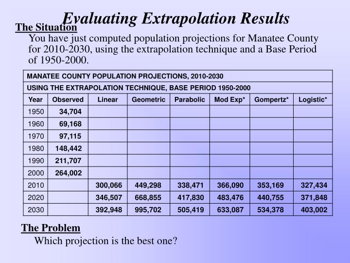
3. Evaluating Extrap Technique Projections There are two general ways to evaluate results from the extrapolation techniques: 1) Quantitative Procedures --Input Evaluation Statistic (CRV) --Output Evaluation Statistics (ME, MAPE) 2) Qualitative Procedures --Eyeball the projections --Evaluate your results with regards to the scenario and assumptions you have made for the study area.

4. Input Evaluation Test • The input evaluation test allows you to determine the curve likely to be the “best fitting” by reviewing the observed data. • This test is performed upon the Observed data (the “Inputs”). • Each of the curves provides a better fit under specific conditions: Linear: When 1st differences are approximately equal Geometric: When differences of logarithms are approximately equal Parabolic: When 2nd differences are approximately equal Mod Exponential: When the ratios of the 1st differences are approximately equal Gompertz: When the ratios of the difference of logarithms are approximately equal Logistic: When the ratio of reciprocal differences are approximately equal

5. The Coefficient of Relative Variation (CRV) • CRV: The standard deviation expressed as a percentage of the absolute value of the mean. CRV = (St dev / |mean|) * 100 • The trick to calculating the CRV is understanding what the underlying assumptions behind each of the curves is and what numbers are used to calculate the standard deviation and the mean. Otherwise the calculations are exactly the same! • The Curve Assumptions: Linear: 1st differences are the same Geometric: Differences of logarithms are the same Parabolic: 2nd differences are the same Mod Exponential: Ratios of the 1st differences are the same Gompertz: Ratios of the difference of logarithms are the same Logistic: Ratios of reciprocal differences are the same • This allows you to compare the “fitness” of the Input Data across each of the curves using a standardized statistic. • When evaluating CRVs, lower values are better.

6. Curve Assumption: 1st Differences are the Same

7. Curve Assumption: Differences of Logarithms are the Same

8. Curve Assumption: 2nd Differences are the Same

9. Curve Assumption: Ratios of the 1st Differences are the Same

10. Curve Assumption: Ratios of the Differences in Logs are the Same

11. Curve Assumption: Ratios of the Differences in Reciprocals are the Same

12. Comparing the Input Evaluation Statistics

13. Output Evaluation Statistics • The output evaluation statistics allow you to compare the observed data with the curve estimates for each of the methods. • These statistics assume that the curve that best fits the observed data will most accurately predict future trends. • These statistics evaluate the extent to which the curve estimates match the observed data. These are quantitative measures of how good the curves actually fit the observed data. • These tests are performed upon the curve estimates (“Outputs”). • Two statistics, both a variation on the same idea: 1) Mean Error (ME) 2) Mean Absolute Percentage Error (MAPE)

14. Mean Error • Mean Error (ME) Mean Error: Sum (Observed - Estimated) / N • The ME is expressed as a value that can be positive or negative. • When evaluating ME’s lower values are better. • The ME are always be about 0 for the Linear Curve, Parabolic Curve, and the “best fitting” Modified Exponential Curve. • Of the three general evaluation statistics (CRV, ME, and MAPE) the Mean Error is the least important because negative and positive values often cancel each other out. • However, the ME is useful because it gives some indication as to the bias of the curve; whether or not the curve is consistently high or consistently low in its fit to the observed data.

16. Mean Absolute Percentage Error • Mean Absolute Percentage Error (MAPE): MAPE: Sum (|Observed - Estimated|)/Observed) / N *100 • The MAPE is expressed as a percentage that offers a direct comparison of the level of error across the various curves. • Like the other two statistics, for the MAPE lower values are better. • The MAPEevaluates the total estimation error, regardless of sign (direction), thereby providing a useful measure of the total variation between observed and estimated data. • The MAPE is deemed the most useful of the three evaluation statistics because it offers a direct comparison of the various curves regardless of the number of observations.

24. Comparing the Output Evaluation Statistics

25. Taken as a whole, our evaluation statistics indicate that three curves offer a potential “best fitting” curve: Modified Exponential, Gompertz, and Logistic. Putting the Puzzle Together • When the three evaluation statistics are viewed together, we see the following:

26. Manatee County Extrapolation Results • The quantitative statistics can only help us so much. They have narrowed our choices, but we need to look at the actual projections to ultimately choose a “best one”.

27. Qualitative Techniques: Eyeballing the Data • While the evaluation statistics paint one picture, an equally important evaluation rests on qualitative methods… methods that rely much more upon the judgment and expertise of the analyst. • The first technique is a very simple one… plot the observed and projected data in a chart and “Eyeball the Data”. • Let’s look at three charts for Manatee County: 1) The Modified Exponential curve 2) The Gompertz Curve 3) The Logistic Curve

32. Qualitative Techniques: Scenario Building • The second major qualitative technique involves what I (and others) term “scenario building”. • At a very basic level, scenario building involves the identification of major ongoing and likely future trends affecting the area of interest and then thinking about how those trends will affect population levels in the future. • What forces will continue to shape Manatee County’s population? --Growth of Tampa Region --Future Vitality or Decline of Bradenton (esp. downtown) --Growth of east Manatee County --Growth of Sarasota --General Health of the State Economy --Others? • We would need to determine which curve identified by our quantitative techniques best fits this scenario?