Download
1 / 14
140 likes | 273 Views
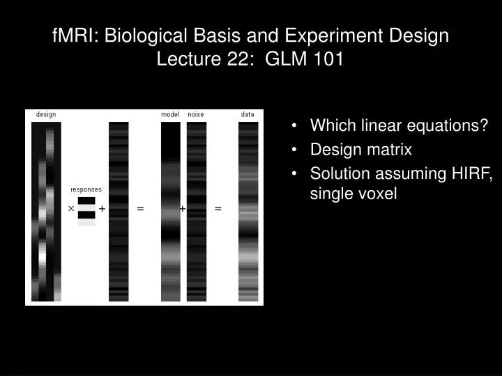
fMRI: Biological Basis and Experiment Design Lecture 22: GLM 101. Which linear equations? Design matrix Solution assuming HIRF, single voxel. +. =. +. =. . Linear algebra. A 1 x 1 + A 2 x 2 + A 3 x 3 + A 4 x 4 = y. is the same as. Ax = y. where. x 1 x 2 x 3 x 4. A =. x =.

E N D
fMRI: Biological Basis and Experiment DesignLecture 22: GLM 101 • Which linear equations? • Design matrix • Solution assuming HIRF, single voxel + = + =
Linear algebra A1x1 + A2x2 + A3x3 + A4x4 = y is the same as Ax = y where x1 x2 x3 x4 A = x = A1 A2 A3 A4
stimulus type time stimulus 1 at t=2 response to stimulus 2 Linear algebra A1,1x1 + A2,1x2 + A3,1x3 + A4,1x4 = y1 A1,2x1 + A2,2x2 + A3,2x3 + A4,2x4 = y2 A1,3x1 + A2,3x2 + A3,3x3 + A4,3x4 = y3 A1,mx1 + A2,mx2 + A3,mx3 + A4,mx4 = ym y1 y2 y3 ym x1 x2 x3 x4 A1,1 A2,1 A3,1 A4,1 A1,2 A2,2 A3,2 A4,2 A1,3 A2,3 A3,3 A4,3 A1,m A2,m A3,m A4,m A = x = y =
Linear model for BOLD in a voxel Ax = y Design matrix, [m x n] - m time-points - n stimulus types Data [m x 1] - response through time Responses [n x 1] - for each stimulus, a scalar (single number) representing how well that voxel responds to that stimulus y1 y2 y3 ym x1 x2 x3 x4 A1,1 A2,1 A3,1 A4,1 A1,2 A2,2 A3,2 A4,2 A1,3 A2,3 A3,3 A4,3 A1,m A2,m A3,m A4,m A = x = y =
Design matrix stim 1 stim 2 stim 3 stim 1 stim 2 stim 3 Matrix form for GLM
Design matrix: assuming shape of HIRF stim 1 stim 2 stim 3 stim 1 stim 2 stim 3 time =
Design matrix: modeling data A stim 1 stim 2 stim 3 BOLD x =
Design matrix, [m x n] - m time-points - n stimulus types Data [m x 1] - response through time Responses [n x 1] - for each stimulus, a scalar (single number) representing how well that voxel responds to that stimulus y1 y2 y3 ym x1 x2 x3 x4 A1,1 A2,1 A3,1 A4,1 A1,2 A2,2 A3,2 A4,2 A1,3 A2,3 A3,3 A4,3 A1,m A2,m A3,m A4,m A = x = y = Solving linear model for BOLD in a voxel measured known Ax = y ... the answer
Solving linear model for BOLD in a voxel Ax = y ATAx = ATy (ATA)-1(ATA)x = (ATA)-1ATy x = (ATA)-1ATy
Solving linear model for BOLD in a voxel x = (ATA)-1ATy y (ATA)-1AT 1 0 0.5 x = =
Linear model for BOLD in a voxel, with noise A(x + ) = y + where A = design matrix [nTimepoints x nStimTypes ], x = concatenated responses [nStimTypes x 1], y = true response [nTimepoints x 1] = noise in data [nTimepoints x 1] = error in estimating response [nStimTypes x 1] Solution: xest = x + = (ATA)-1AT (y + ), so = (ATA)-1AT
A(x + ) = y + xest = x + = (ATA)-1AT (y + ) 0.96 -0.18 0.49 y + xest = 1 0 0.5 x = A*xest
Example: block design with linear trend Design matrix: Solution: x = [ 1 ; 0.2]; xest = [ 1.01 ; 0.24 ]
Example: block design with linear trend Design matrix: Solution: x = [ -0.5 ; 0.2]; xest = [ -0.46 ; 0.25 ]