Download
1 / 30
300 likes | 478 Views
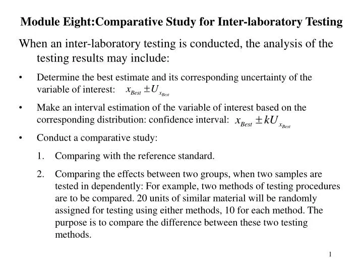
Module Eight:Comparative Study for Inter-laboratory Testing When an inter-laboratory testing is conducted, the analysis of the testing results may include: Determine the best estimate and its corresponding uncertainty of the variable of interest:

E N D
Module Eight:Comparative Study for Inter-laboratory Testing • When an inter-laboratory testing is conducted, the analysis of the testing results may include: • Determine the best estimate and its corresponding uncertainty of the variable of interest: • Make an interval estimation of the variable of interest based on the corresponding distribution: confidence interval: • Conduct a comparative study: • Comparing with the reference standard. • Comparing the effects between two groups, when two samples are tested in dependently: For example, two methods of testing procedures are to be compared. 20 units of similar material will be randomly assigned for testing using either methods, 10 for each method. The purpose is to compare the difference between these two testing methods.
3. Comparing the changes of a response before and after (or with/without) a treatment is performed. For example, to test the poison of a chemical compound with and without an additional additive in ten labs. Each compound is divided into two sub-samples. Each lab test the pair of the compound, one with additional additive, he other without. The difference between each pair tested by a lab is due to the additive. Note, in this comparative study, each pair of sub-samples are the same or very similar. This is a paired sample problem. • 4. Comparing the effects among several groups, when a treatment has more than two levels. This type of comparative studies are common in inter-laboratory testing. For example, one is interested in studying the compressive strength of concrete using five different formula. Ten specimen are produced using each formula. The compressive strengths are tested. This is a one-factor experiment with five factor levels. Our interest is to compare their strength and to determine which formula gives the highest strength. If the only difference of these formula is the dosage of an additive, ranging from 1%, 1.5%, 2%, 2.5% and 3%. Then, in addition to compare the strength among the formula, we can also fit a prediction model to determine the dosage level that results the maximum strength.
5. In many experiments, there may be more than one factor. The study is not only understand the effect of each factor, but also to study the interaction effect between two factors. This is a multifactor study. For example, For the compressive strength of concrete testing study, in addition to the five levels of formula, in the process of concrete formation, the temperature is another critical factor. We should consider both formula factor and temperature factor when producing the specimen for strength test. Suppose we would like to test for three levels of temperature. We have 5x3 two factorial design. For each treatment combination, four specimen are produced. We have a total of 3x5x4 = 60 specimen for strength testing. We are interested in studying comparing the strength among different formula, among different temperature, and the strengths among different formula for each temperature level. 6. Another type of study in lab testing is to study the variance components of factors for the purpose of identifying factor levels that will reduce variability of response variable. For example, in a metal alloy casting process, each casting is broken into small bars that are used for other applications. The tensile strength of the alloy is critical to its intended use. There is a specification of the strength. If variation of the strength is excessively large, this means a large amount of bars will not meet the specification limits. An experiment can be designed to identify factors and their level combinations that will produce bars with small variability. This is a variance component problem.
In this module, we will discuss the type of comparative studies: 1, 2 and 3. In Module Ten, we will discuss the comparative study four, the one-factor design and analysis. And in Module Eleven we will focus on comparative 5, multifactor designs and analysis. Module Twelve will study the Variance Components problems.
Comparative Study One: Comparing testing results with a given reference or a given standard • In a lab testing study, one may be be interested in making a comparison of the testing results with a given standard or a reference measurement. The following steps may be applied to plan such a study: • Identify the given standard or reference measurement, and make sure the resource that developed the standard meet your purpose. • Set up an adequate lab testing environment and testing procedure. • The operator of the testing should be adequately trained to reduce unexpected errors. • Plan the experimental procedure, determine the number of experimental runs to be conducted. • Prepare the needed experimental units, and make sure these units are as homogeneous as possible. • Conduct the lab testing and carefully collect the data of interest. It is a good practice to record any special events occurred during the testing.
Now, a data set is collected, and we would like to make a comparison with a given reference. Steps for this analysis may include: • Carefully check the data for unusual measurements that may be due to systematic error or special causes – Techniques for detecting outliers can be applied here. • Compute descriptive summaries and graph a histogram, box plot for identifying outliers and normal probability plot for checking the normality assumption. • If there is a serious violation of normality assumption, one may choose to make a data transformation. If there are outliers, one should go back to check the possible special causes, and decide to keep or drop these outliers before the analysis. • The comparison is the one-sample test. Here is the procedure to conduct the comparison.
One-sample t-test for comparing the testing results with a given reference. Example: The brightness of a certain type of paper is defined in the scale of 1 to 100. A reference of the brightness of the type of paper is at the scale 60. A lab is experimenting a new process for producing the type of paper, and would like to test its brightness to see if the paper meet the required brightness. A random sample of 30 sheets are chosen and tested by a lab. Here is the collected data: A quick eye check immediately identify a value of 42, which a much smaller than the rest. We first draw a box plot and a normal probability to identify outliers and to check the normality assumption.
Reviewing the records from the lab testing, it is noticed that the paper given ’42’ was due to a special cause of wrong timing in a testing process. It is therefore removed from further analysis. • The normality test appears data follow normal curve very well.
The concept and Procedure for performing the one sample t-test When we are conducting a hypothesis test for comparing with a given reference, there are usually two choices; one is the hypothesis we intend to establish in our study, the other is the opposite. In order to make the procedure of testing easier, we define these two hypotheses: H0 and Ha. Ha is the one we intend to establish. For this paper brightness test, our Ha is the actual average brightness of the paper is significantly different from the given reference. Typical notation for the hypotheses are: For the paper brightness study, we have: Q: When.how do we decide to take H0 or Ha ? As we see, if the average of the sample data is either much larger or much smaller than 60, we will choose Ha; otherwise, we choose H0.
Q: But, how far is far enough to make such a conclusion? If the sample average is, say 59.5 or 60.4, then, we would not conclude it is far enough to conclude Ha. Therefore, we will need two critical average brightness, , so that when the sample average obtained from the sample data is beyond these two values, we will conclude Ha, that is, the brightness is of the paper is significantly different from the reference brightness, 60. Q: How to determine the two critical values? This can be answered by bringing in the distribution of . The following distribution is the distribution of under H0. Our common experience suggests that the probability of rejecting H0 should be small, so that, only when the sample average is much far away from 60, we will conclude Ha. Therefore, a typical probability for rejecting H0is 5% or 1%. Standardized form of is used for making proper comparison, which is the t-distribution. a/2=.025 a/2=.025 60 Reject H0 Accept H0 Reject H0 -t(a/2, n-1 t(a/2, n-1
Procedure for conducting one-sample t-test: • Set up H0 and Ha • Determine the rule for rejecting and accepting H0 regions based on the type of hypothesis rule based on the t-distribution. • From the sample data, we compute the t-value from the sample average: • 4. Compare the tobserved with the critical t-values , -t(a/2, n-1 and t(a/2, n-1)from the t-table to determine if tobserved falls in the Acceptance or in the Rejection region. NOTE: Computer output gives us both the tobserved and the observed level of significance, namely, the p-value. The p-value for this two-sided test is 2P(t > |tobserved|) And the decision making based on p-value is : P-value < a , then, we reject H0, that is decide to take Ha P-value a , then, we conclude H0
Right-side and Left-side tests • Ha is the hypothesis we intend to establish. Therefore, in applications, other tha two-side tests, there are two common hypotheses: • Right-side test : • Left side-test. • How to choose the test for our need? • If our intension is to find out if the sample mean is much larger than the reference value or not, right-side test should be applied. For example, if the reference value of the brightness of paper, 60, is the minimum. Our goal is to decide if the new process produces significantly brighter paper or not. • If our intension is to find out if the sample mean is much lower than the reference value or not, right-side test should be applied. For example, if the reference value of the brightness of paper, 60, is the maximum allowed. Our goal is to decide if the new process produces significantly less bright paper or not. • If our intension is to find out if the sample mean is much lower than the reference value or not, right-side test should be applied. For example, if the reference value of the brightness of paper, 60, is the given standard. Our goal is to decide if the new process produces significantly different brightness of paper or not.
Hands-on Activity: Comparative Study with A given Reference In testing the tensile strength of a new type of concrete, the goal is to make sure that the tensile strength meets the minimum of 300 psi. A lab is assigned to test this new concrete. 20 samples are tested. The tensile strengths are : Perform an appropriate test to determine if the new type of concrete meets the minimum tensile strength of 300 psi.
Comparative Study for Inter-laboratory Testing : two-group cases • Using the example of brightness of paper, there are many situations that the testing may involve with two groups of treatment. Here are some possible situations: • when chemical component is changed, the brightness could be changed dramatically. A comparative study can be planned to compare the effect of two different levels of this chemical component. • When papers are tested by two different labs, there may be between-lab differences. Such difference should be controlled to minimize the systematic error of a given lab when testing the same material using the same testing procedure. • When papers are testing using two different testing procedure, it is important to identify the difference between these two testing procedures. A comparative two-group study may be to compare the difference of two types of material, two different treatments , two testing procedures, or difference between two labs. We now discuss a method for making the two-group comparison. Similar to the comparison between a given reference and a sample data, if is important to keep in mind that we need to conduct outlier analysis and distribution checking.
Add Level A component Test n = 15 pairs. Each pair are tested together Specimen is split into two sub-samples Add Level B component Add Level A component Test n = 15 units Test n = 15 units Add Level B component The issue of designing experiments for two-sample comparative study Consider the example of comparing the reaction of a chemical component in a lab testing Treatment : Two levels of chemical component. We will discuss two types of designs for experiment: • Design A – Paired sample design: The units assigned to two treatment each time are very similar, since they are from the same specimen. • Design B-Independent sample design: Each treatment is assigned to 15 units, which are independent of the other treatment. NOTE: a paired-sample comparison is usually referred to Before/After Treatment or Pre/Post Treatment experiment. The variable of interest is observed before and after a treatment. This type of design occurs often in testing the effect of c treatment along the time domain. For example, one my be interested in studying the chemical residue for 5 day, 10 days after the chemical is sprayed to a certain vegetable.
NOTE: a paired-sample comparison is usually referred to Before/After Treatment or Pre/Post Treatment experiment. The variable of interest is observed before and after a treatment. This type of design occurs often in testing the effect of c treatment along the time domain. For example, one my be interested in studying the chemical residue for 5 day, 10 days after the chemical is sprayed to a certain vegetable. Time Treatment: Spray the chemical to n randomly chosen subjects. Test the residue five days after from the subjects Test the residue ten days after from the same subjects Treatment is given. Eg, a diet treatment for three months Time Before diet treatment: observe weight, BMI, age, Gender, etc, from each subject Three months after, observe weight, BMI, etc, from the same subject. Hands-on Activity For the same study, one can design a two-independent sample study as well. Design a two independent sample study for studying the chemical residue, and discuss the advantage and disadvantage of paired-sample Vs independent sample designs.
The difference between Experiment A and B is: Samples obtained from experiment A can be considered as 15 pairs, each pair is sampled from the sub-group. Possible sources that may introduce the error is the same for two samples except the levels of component. The experimental units are similar. Samples obtained from Experiment B are two independent samples. Each is obtained from the process that is independent from the other process. Possible sources that may introduce errors include not only the levels of components but also the differences of the processes. Therefore, the paper units for testing the brightness may have higher variation. Analyses of data resulted from these twp experiments are different. Experimental A is a paired sample problem, while B is an independent sample problem. Hands-On Activity From the projects you have conducted, identify a paired sample project and one for independent sample project.
Analysis of Paired Sample Problem Consider the experiment for testing the chemical residue. Experiment: 15 pots of a certain vegetable are used as the experiment units. The residue is measured and recorded five days and ten days after the spray. X: the residue five days after the chemical treatment. Y: the residue ten days after the chemical treatment. Testing Procedure: Each residue is the average of the residues of two specimen taken from the same plot for the purpose of reducing random error. For each pot, the residues are observed five days and ten days after. Hence the difference between Y-X is the residue reduction in the five days of time period. To understand if the reduction of residue is statistically significant, we can then perform a one-sample test based on the difference, d. The hypothesis is:
Recall: To perform a one-sample t-test, we need: The following is the output from Minitab Paired T for 10 days - 5 days N Mean StDev SE Mean 10 days(y) 15 58.600 2.849 0.735 5 days (x) 15 62.200 2.731 0.705 Difference (d) 15 -3.600 3.376 0.872 95% CI for mean difference: (-5.470, -1.730) T-Test of mean difference = 0 (vs not = 0): T-Value = -4.13 P-Value = 0.001 • Based on the p-value = .001 < 5%, we can conclude that the residue reduction is statistically significant at a = 5%. The average reduction is 3.6 based on data from 15 pots. • The confidence interval at 95% is given by • –5.47 to –1.73. That is the 95% sure that the uncertainty of the residue is
Analysis of Two-independent Samples Problem Consider the experiment for testing the chemical residue. We can design a two-independent sample experiment for the residue study. Experiment: 30 pots of a certain vegetable are used as the experiment units. 15 pots are randomly chosen for the 5-day residue testing. The other 15 are for the 10-day residue testing. X: the residue five days after the chemical treatment from 15 randomly selected pots. Y: the residue ten days after the chemical treatment from the other 15 pots. Testing Procedure: Each residue is the average of the residues of two specimen taken from the same plot for the purpose of reducing random error. NOTE: This design is appropriate if each pot can only be applied for one residue testing. For each pot, the residue can only be measured either five days or ten days after. The assignment of pots to residue testing is random, and thus, there are considered independent. The difference between Y-X no longer reflects the residue reduction, but also include the pots difference.
The residue after 5-days is a population with it’s mean m1and variance, s12. Similarly, the residue after 10-days is a different population with it’s mean m2and variance, s22. Our purpose is to compare if m2 is statistically lower than m1. This is a left-side test: Ha is concluded if the corresponding sample mean difference, is indeed much lower than zero. How much less from zero is considered significant? Similar to the one-sample problem, we need to determine the distribution of Or equivalently, the distribution of the standardized form, NOTE: Most of statistical hypothesis problems or estimation problems require the distribution form of the best estimate of the variable of interest. This is usually accomplished by finding the distribution of the standardized best estimate. This is true for any test involves t-distribution, chi-square distribution, as well as F-distribution, and so on.
What is the distribution of ? How to determine ? Based on statistical theory, the t-distribution holds when the samples are randomly chosen from each population. The quantity is the uncertainty of the the mean difference. The way for determining depending on the sample sizes and if the variances of two populations are homogeneous or not. When the population variances are not equal, then is given by:
When the population uncertainties can be assumed equal, that is, we can combine two samples together to obtain a better estimate of the common measurement uncertainty for : • obtain the pooled estimate of the common variance, s2 ,by: • Compute SE of : The 100(1-a)% confidence interval for can be determined by:
To test if population mean m2statistically different from (greater or less than) the population mean m2. • We apply the t-test by: • Compute t-value: • Compare tobs with the critical t-value: • Or when computer software is available, the p-value is used for decision making. The same rule is applied when using p-value, regardless what type of test: • If p-value < a, then, reject H0, and conclude Ha
Case Example: A chemical residue study Purpose: To compare if chemical residue is significantly reduced ten days after with 5 days after. Experiment: 30 pots of a certain vegetable are used as the experiment units. 15 pots are randomly chosen for the 5-day residue testing. The other 15 are for the 10-day residue testing. X: the residue five days after the chemical treatment from 15 randomly selected pots. Y: the residue ten days after the chemical treatment from the other 15 pots. Testing Procedure: Each residue is the average of the residues of two specimen taken from the same plot for the purpose of reducing random error. Variable Treatment N Mean Median StDev SE Mean Residue 5-days 15 62.20 63.00 2.731 0.705 10-days 15 58.60 59.00 2.849 0.735
Diagnosis of assumptions: • Both samples follow normal. • Variances are similar.
Two-Sample T-Test and CI: Residue, Treatment (Without assume equal variances) Treatment N Mean StDev SE Mean 1 15 62.20 2.73 0.71 2 15 58.60 2.85 0.74 Difference = mu (1) - mu (2) Estimate for difference: 3.60, 95% CI for difference: (1.51, 5.69) T-Test of difference = 0 (vs >): T-Value = 3.53 P-Value = 0.001 DF = 27 Note: DF = 27 is computed to adjust the unequal variances Two-Sample T-Test :Residue, Treatment ( assume equal variances) Difference = mu (1) - mu (2) Estimate for difference: 3.60 T-Test of difference = 0 (vs >): T-Value = 3.53 P-Value = 0.001 DF = 28 Both use Pooled StDev = 2.79 Note: sp is used as the common s.d.
Conclusion: The s.d.’s are similar. Levene’s test of uniformity of variances shows p-value = .835. We can use either t-test to test the hypothesis ‘If the residue 10-days after is significantly reduced from 5-days after. Two t-test results (assuming/not assuming equal variance) give the same conclusion: P-value < 5%, therefore, the reduction of residue from 5-days to 10-days after the chemical spray is statistically significant.
Hands-on Activity Perform the two-independent sample test manually, and compare with the computer output.