Download

1 / 58
580 likes | 651 Views
Planck Diffuse Component Separation TWG2.1 Review. coordinators Carlo Baccigalupi, Simon Prunet, Michael Linden-Vornle Paris, November 24, 2001. Members & Criticalities Results & Activities, Oct.2002 Results & Activities, Nov.2003 Work Group Activities Interactions with other TWGs

E N D
Planck Diffuse Component SeparationTWG2.1 Review coordinators Carlo Baccigalupi, Simon Prunet, Michael Linden-VornleParis, November 24, 2001
Members & Criticalities Results & Activities, Oct.2002 Results & Activities, Nov.2003 Work Group Activities Interactions with other TWGs Near Future … Spectral Matching Flexible MEM & COBE FastICA & COBE systematics removal FastICA & polarisation IFA Spatial Matching Harmonic FastICA TWG2.1 Review Contents
TWG2.1 Members Mark Ashdown, Vladislav Stolyarov(CPAC, Cambridge) Carlo Baccigalupi, Francesca Perrotta (SISSA, Trieste) James Bartlett, Alain Bouquet, Jacques Delabrouille, Yannick Giraud-Heraud, Jean Kaplan (CdF, Paris) Luigi Bedini, Emanuele Salerno, Anna Tonazzini, Ercan Kuruoglu (IEI, Pisa) Carlo Burigana, Lucia Popa (TeSRE, Bologna) Krzysztof Gorski (MPA, Munich) Eric Hivon, Jeffrey Jewell, Steve Levin (JPL, Pasadena) Patrick Leahy (Jodrell Bank) Michael Linden-Vornle (DSRI, Copenaghen) Davide Maino (Milano) Simon Prunet (IAP, Paris) Benjamin Wandelt (Princeton)
TWG2.1 Criticalities • Unique package • Flexibility • Maps, Harmonics & TODs • Blind & non-Blind merging • Polarisation • Complementarity • New techniques & development • Test with incoming CMB data
TWG2.1 Criticalities status at the Santander meeting, Oct. 2002 • Unique package • Flexibility results,ongoing • Maps, Harmonics & TODs results,ongoing • Blind & non-Blind merging results,ongoing • Polarisation ongoing • Complementarity results • New techniques & development ongoing • Test with incoming CMB data results,ongoing
TWG2.1 Criticalities status at the Paris meeting, Nov. 2003 • Unique package • Flexibility results+,ongoing+ • Maps, Harmonics & TODs results,ongoing+ • Blind & non-Blind merging results+,ongoing+ • Polarisation results • Complementarity results • New techniques & development results,ongoing+ • Test with incoming CMB data results+,ongoing+
TWG2.1 Results Review status at the Santander meeting, Oct. 2002 Flexibility: indications of stability against spectral index variation of ICA based techniques (Baccigalupi et al. 2002); effective removing of instrumental noise patterns (Delabrouille, Patanchon, Audit 2002; built-in non-stationary noise techniques (Kuruoglu 2002) Maps, Harmonics & TODs: MEM & WF matching with the harmonic space analysis (Stolyarov et al. 2002, Challinor et al. 2002; Prunet et al. 2001) Blind & non-Blind merging: blind estimation of separation matrix & Wiener filtering (Cardoso et al. 2002); constraining elements of the separation matrix & source distributions (Bedini, Salerno, Tonazzini 2001) Complemenratiry: results of matching MEM & MHW (Vielva et al. 2001) New techniques & development: EM algorithm & IFA technique (Snoussi et al. 2001, Bedini, Salerno, Tonazzini 2001)
TWG2.1 Activity Review status at the Santander meeting, Oct. 2002 Flexibility: preparing study of FastICA stability against principal systematics; parameter adjustment by spectral matching Blind & non-Blind merging: testing IFA on simulations Polarisation: application of FastICA to polarised maps Complementarity: matching MHW with FastICA New techniques & development: imprint on non-Gaussianity Of MEM based component separation Testing with incoming CMB data: spectral matching on Archeops, FastICA & MEM for COBE, preparing for WMAP
TWG2.1 Results Review status at the Paris meeting, Nov. 2002 • Spectral Matching (Delabrouille et al. 2003) • Flexible MEM & COBE (Barreiro et al. 2003) • FastICA & COBE (Maino et al. 2003) • Systematic removal (Delabrouille et al. 2002) • FastICA & polarisation (Baccigalupi et al. 2003) • Spatial Matching (Bedini et al. 2003)
TWG2.1 Activity Review status at the Paris meeting, Nov. 2002 • IFA testing (Kuruoglu et al. 2003) • SM on Archeops data (Delabrouille et al. 2003) • Harmonic (Maino et al. 2003) • FastICA & WMAP • …
Spectral Matching Concept • Cl of the components to recover, mixing matrix, even noise considered as parameters • fit those parameters by matching with real data in the harmonic domain • control degeneracies with available priors (CMB frequency scaling, approximate template and frequency scalings for foregrounds, …)
Flexible MEM & COBE • Priors are only partially known when dealing with real data • make MEM flexible by running with many priors and estabilishing the ``Goodness” of the results by matching with real data • Perform Monte Carlo simulations to quantify the effect of systematics and apply to real data
Astrophysical Component Separation on COBE-DMR 4yr data with FastICA D.Maino, A.J. Banday, C. Baccigalupi, F.Perrotta, K.M.Grski MNRAS, 2003, 344, 544
Introduction Present and future CMB experiments (WMAP and Planck) will map the microwave and sub-mm emission over the entire sky with high resolution and sensitivity The goal is to extract genuine CMB anisotropy from which contruct the angular power spectrum and constrain cosmological parameters Several contaminant emission both from out Galaxy (synchrotron, free-free and dust) and from extra-galactic sources (radio- and IR-galaxies, SZ effect,...) It is crucial to identify and remove such components with high accuracy and reliability
Component Separation Approaches “non-blind” algorithms (Weiner Filter, Maximum Entrophy Method): they need “priors” on the signal to be separated (frequency scalings, power spectra, etc.) “blind” algorithms (Independent Component Analysis, Expectation Maximization): they do not assume any “priors” on physical properties of signals but expliot their different statistics (ICA) or spectra (EM)
Component Separation Problem - I sky signal is the superposition of N different processes for which the spectral and spatial dependences are factorized as: we have M channels with specific PSF B(r,). Suppose B is both shift invariant and constant in the bandwidth t()
Component Separation Problem – II • assume that B is independent from frequency i.e. each channel has the same beam pattern • we want to determine s and A given the data x • in general the problem is not solvable if additional information is not provided. Different algorithms work with different information
FastICA algorithm - I the signal s are independent random processes, all signals, but at most one, have NG distribution, independent components are extracted maximizing a suitable measure of NG, the model is noisy so we need a “robust” measure of NG and this is the Neg-Entropy, find a matrix W for which the transformed variables y=Wx are in fact independent,
FastICA algorithm - II assume we know the noise covariance matrix N “rotate” variable along Principal Components (PC) separation matrix W is estimated row-by-row i.e. one component at a time
FastICA algorithm - III • choose an initial vector w (randomnly) • update it by • here g is a non-quadratic form that approx. NegEntropy: g(u) = u3, g(u)=tanh(u), g(u)=u exp(-u2) • normalize wnew to be a unit vector • compare wnew with the old vector;if converged start another row; if not go to step #2 • the k+1th row is searched in a sub-space orthogonal to the first k rows (Gram-Schmidt rule)
FastICA algorithm - IV FastICA gives coefficients for a linear combination of the input data that finds independent components these coefficients are found in a non-linear way from these coefficients we can derive spectral indeces of the components with the same coefficients we can estimate the signal-to-noise ration in the extracted components: useful if we want extract cosmological parameters
Application to COBE-DMR 4yr data DMR observed full-sky at 31.5, 53 and 90 GHz. With 2 separated channels (A and B) measured temperature differences between point 60° apart each frequency has the same beam shape with 7° FWHM S/N is poor: 0.5,1.5 and 1 when combining A and B at 31.5, 53 and 90 GHz instrumental noise is white and Gaussian but not uniformely distributed: variations by a factor of 4 (6) are observed at 53 and 90 GHz (31.5 GHz) noise distribution at 31.5 is different from that at 53 and 90 due to a known systematic effect
Impact of noise distribution and amplitude what is the impact of noise distribution on components?
Testing Noise Distribution • we run ~ 3000MC simulation of fake CMB sky (Qrms=18uK and n=1) with DMR noise as follows • DMR nominal noise amplitude; • uniform noise distribution with nominal mean ampl. • uniform noise distribution with ampl. lower by a factor of 4 • for each simulation we extract CMB component with all 3 non-quad. form of FastICA and evaluate spectral index and power spectrum • in each case we consider all 3 DMR channels and only 53 and 90 GHz.
Simulations Results - I expected CMB spectral index between 90 and 53 GHz:0.876
Simulations Results - II including 31.5 GHz yields a spectrum with less power FastICA is sensible to differences in noise distributions
Extracting Cosmological Parameters we expand the extracted CMB component in spherical harmonics on the cut-sky obtaining a set of coefficients c we know the dependence of signal (CMB) correlation matrix C from cosmological parameters p we can estimate noise in the reconstructed component to get the noise covariance matrix N
Qrmsand n cosmological parameters FastICA can extract CMB component consistent with G96 without foreground correction FastICA is not able to extract any foreground from DMR data alone
Adding “priors” on foregrounds we add 2 extra channles: the Haslam 408 MHz map and the DIRBE 140m map as templates for the diffuse galactic radio emission and diffuse infra-red emission noise in the extra chennels is small compared to DMR FastICA returns 4 components: the S/N will guide us to the physical ones
Results – Foreground Emissions - I “foreground” components closely resemble Haslam and DIRBE maps but rs ~ 0.9 some features of one components appear as “ghost” in the other one. This is probably due to: i) large angular scale correlation between foreground; ii) low S/N at high galactic latitudes;iii) large smoothing with DMR beam the aliasing is dependent on the non-quad. form however CMB is well reconstucted and remains clean from galactic emission
Results – Foreground Emissions - II FastICA can give information on foreground by means of the coefficients of the matrix W which states the linear combination of the input data to obtain final components these “weights” can be interpreted as correlation coefficients between templates and DMR data we include a new H emission (Dickinson et al. 2003) as free-free templates run FastICA at each DMR frequency with 3 templates we calibrate which form is best suited using fake skies with foreground using results from Banday et al. (2003) and ~10,000 noise realisations -> p and g are consistent
Results – Foreground Emissions - III general good agreement with Banday et al. (2003) with an independent approach (correlation analysis in harm.) there is a clear evidence of a component correlated with DIRBE which is the major foreground emission at 31.5GHz which is the nature of this anomalous dust component? We subtract from data model 7 of FDS: 2 dust components with T1=9.6K and 1=1.5 and T2=16.4K and 2=2.6
Results – Foreground Emissions - IV we investigate spectral behaviour fitting data with Anorm(/0)-, with Anorm in K/(MJy/sr-1) and 0=31.5 GHz
Conclusions - I FastICA can work on real data even with low S/N and can also deal with non-uniform noise distribution. However these have to be similar between different channels Good agreement on Qrms and n extracted by FastICA with previous analysis with independent methods Foreground emissions have too low S/N to be extracted from DMR data alone: adding “priors” helps in CMB reconstruction but not in the foreground components
Conclusions - II • information on foregrounds can be extracted from “correlation analysis with DMR data and templates: interesting results in agreement with Banday et al. (2003) with independent approach • data seems to indicate an anomalous dust correlated component which is well fitted by a power-law with a spectral index ~2.56 different from the expected free-free • blind component are promising and application to WMAP is on-going
Systematics Removal: an example • Long spatial correlations in noise can be seen as a signal, seen in different timeline portions in detectors at different frequencies, • in the Fourier space, detectors scanning the same circle see the noise shifted by a phase factor, • include the noise in the components to separate and extract.
Component Separation & Polarisation • The foreground contamination is worse and priors are weaker in polarisation with respect to total intensity • exploit the statistical difference in background and foreground signals, and the great detail of high resolution maps, in ideal conditions • if the nominal performance is satisfactory, check degradation with systematics
Harmonic Approach to Components Separation with FastICA D.Maino, A.J.Banday, C.Baccigalupi, F.Perrotta, M.A.J.Ashdown, K.M.Górski
Motivations one of the main limitation of FastICA in real (pixel) space is the requirement of equal beam width in each frequency channel current and future CMB experiments will map the sky at several frequencies using optical systems (telescopes) which produce different beam shapes in different locations on the focal plane beam convolution in harmonic space is a simple multiplication: much more easely handable than convolution in real space
Component Separation Problem - I • sky signal is the superposition of N different processes for which the spectral and spatial dependences are factorized as: (1) • we have M channels with specific PSF B(r,). Suppose B is both shift invariant and constant in the band t() (2)
Component Separation Problem - II • it usual to expand a field on the sphere in spherical harmonic functions. Rewriting Eq(1) in vector form and expanding in harmonics we found (3) • the covariance matrix could be written and becomes (4) where Xlis the power spectrum of the observed signals. • different angular resolution are treated by dividing each side by Bl2.
FastICA algorithm - I the signal s are independent random processes all signals, but at most one, have NG distribution independent components are extracted maximizing a suitable measure of NG the model is noisy so we need a “robust” measure of NG and this is the Neg-Entropy find a matrix W for which the transformed variables y=Wx are in fact independent
FastICA algorithm - II assume we know the noise covariance matrix N “rotate” variable along Principal Components (PC) separation matrix W is estimated row-by-row i.e. one component at a time
FastICA algorithm - III • choose an initial vector w (randomnly) • update it by • here g is a non-quadratic form that approx. NegEntropy: g(u) = u3, g(u)=tanh(u), g(u)=u exp(-u2) • normalize wnew to be a unit vector • compare wnew with the old vector;if converged start another row; if not go to step #2 • the k+1th row is searched in a sub-space orthogonal to the first k rows (Gram-Schmidt rule)
FastICA algorithm - IV FastICA gives coefficients for a linear combination of the input data that finds independent components these coefficients are found in a non-linear way from these coefficients we can derive spectral indeces of the components with the same coefficients we can estimate the signal-to-noise ration in the extracted components: useful if we want extract cosmological parameters