Download
1 / 30
300 likes | 395 Views
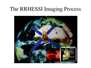
The HESSI Imaging Process. How HESSI Images.

E N D
How HESSI Images HESSI will make observations of the X-rays and gamma-rays emitted by solar flares in such a way that pictures of the flares can be reproduced in data analysis programs in computers on the ground. The purpose of this presentation is to explain how HESSI makes these observations in space, and how the information is used on the ground to create these images.
A First Look at the Instrument • This image is a layout of HESSI’s nine detectors. • The precise orientation of the grids in space is recorded using the Solar Aspect System (SAS) and the Roll Angle System (RAS).
First, one must consider a steady point source on the Sun • Photons are emitted from the source in all directions. HESSI is only concerned with those that reach the instrument.
All photons that reach HESSI can be considered as traveling on parallel paths since the Sun is so far away (93 million miles or 1.5 x 10¹¹ m) compared to the diameter of the HESSI grid tray (~1 m). The largest angle between any 2 photons detected would be 1m/1.5 x 1011m x 360/2 pi degrees = 1.2 x 10⁻⁶ arcseconds
The resolution of HESSI’s finest grids is 2 arcseconds • This is several orders of magnitude greater than the possible 1.2 x 10⁻⁶ arsecond angle between photons
Now to the Animations… • A series of Flash animations have been created to more easily explain the HESSI Imaging process. Ranging from the collection of data to the back projection imaging algorithm
Components of Animations FrontGrid Rear Grid Detector These are the main parts of the Flash animations that illustrate how HESSI’s rotating grids work.
All Nine Grids RotatingPoint Source Located Exactly on the Spin Axis • Next, consider how the grid pairs modulate a parallel beam of photons • Imagine yourself riding along on one of the photons being emitted from the source • The accompanying animation shows what you would see assuming you were traveling exactly along the HESSI spin axis.
All Nine Grids RotatingPoint Source Located Exactly on the Spin Axis • Only the slats of the front grid (in red) would block your view of the detectors (in yellow) • The thermal insulation blankets and the cryostat cover (not seen) used to keep the instrument cool are transparent to all but the lowest energy X-rays.
Another Consideration… • As photons travel from the front grid to the rear grid, HESSI is rotating at 15 rpm. However, the time it takes a photon to travel this length is negligible since the distance between grids is only 1.55 m and the photon is traveling at the speed of light (186,000 miles per second or 3 x 1010cm s‑1). It only takes 5.2 x 10⁻⁹ s for light to travel 1.55m. As shown by the equation: (1.55 * 102)/(3 * 1010)s = 5.2 * 10-9s • At the 15 rpm rotation rate, even the grids near the edge of the trays move a very small distance in this time (2 pi x 50 x 5.2 x 10‑9/4 cm = 0.004 microns) compared to the finest slit width (20 microns).
Source Exactly on the Spin Axis: Single Grid Pair • Shows what a photon traveling along the HESSI Spin Axis would see • No modulation of the visible portion of the detector • All detectors record a steady rate of photons equal to a fraction of those that passed through the front grid.
Source Exactly on the Spin Axis: Single Grid Pair • If front and rear grids were “in phase,” 50% of photons would be detected • Front and rear grids are offset slightly in reality • Exact offset will be determined from the first flares detected
Source Offset From the Spin Axis: Single Grid Pair • Front and Rear Grids no longer appear concentric • Area of detector (yellow) visible through both grids changes with time indicating that the detector counting rate is modulated in time. • Because the front grid (red) appears above the rear grid (blue), the source is below the spin axis on the Sun • The next slide illustrates this point further
All Nine Grids Rotating Source Offset from the Spin Axis • This is the view of both grid trays and all nine detectors from a point on the Sun below the HESSI spin axis
Transmission Fraction • The area of each detector (yellow) seen through the front and rear grids tells you how many of the photons riding along with you in the virtually parallel beam from your common point source will be recorded by HESSI at any given time. • The number of photons on your parallel beam that will be recorded by HESSI changes between 50% of the photons (when the slats of the front grid do not block any part of the rear slits or openings) and no photons (when the slats of the front grid completely cover the slits of the rear grid). 50% transmission 0% transmission
Another Way to Look at HESSI’s Rotating Grids • The accompanying animation is another way to look at the modulation of the visible portion of the detector • It shows how the visible area of the detector modulates with time and how the rate of that modulation also changes
Yet Another Way to Look at HESSI’s Rotating Grids • This animation strictly shows the area of the detector visible at any time excluding the rotation that actually occurs to simplify matters. • This is the sole purpose for this animation, because HESSI does not image by moving the front grid vertically or horizontally with respect to the rear, they rotate about their centers.
Light Curve • Graph generated by the modulation of the area of the detector visible to the source as a function of rotation angle • It takes 4 seconds to generate a lightcurve (15 rpm gives one 360 degree rotation every 4 sec) • Illustrates the transmission fraction (the fraction of the detector area visible to the incoming photons) changing between 0 and 0.5
Back Projection • Animation shows the possible paths along which a detected photon could have traveled. • Tracing these directions back to the Sun produces a probability map of the sky, lines where photons could and could not have originated at any given time.
These 5 animations represent the back-projection process by which the information about the modulated signal seen by one of the HESSI detectors is transformed into an image of the flare as seen in X-rays or gamma-rays.
This box represents the area of the detector seen by the source: the white is the portion of detector, black is the combined area of the front and rear grids that blocks a certain portion of detector, leaving between 0 and 50% of the detector visible to the source
This box shows what the detector sees as a function of time: white = maximum transmission, black = no transmission.
This box shows the light curve of the time variation of the fraction of the X-ray and gamma-ray photons that pass through the two grids and reach the detector.
This box contains a probability map of the Sun showing where photons could and could not have originated at a specific time during the rotation. • In the bottom left hand corner of the box is the location of the point source. The white areas have maximum probability and the black areas have minimum probability that a photon detected at each particular time could have come from those locations on the Sun.
These boxes show the accumulation of probabilities as the spacecraft rotates and the final reproduced image of the source • The “ghost” source (upper right-hand corner) appears because the same modulation pattern would have occurred for a source on the opposite side of the spin axis (Exactly 180 degrees with respect to the center). In practice, the slight movement of the satellite’s spin axis over time will blur the ghost source but leave the true source with full intensity.
Combining Several Point Sources to Create a Solar Flare • The image on the left represents a test flare reproduced using the HESSI Data Analysis Software • Point sources were placed together to form two flares in the shape of a “B” and the number “3”