Homework on ANOVA

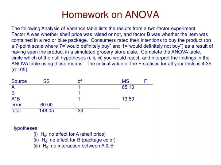
1. Homework on ANOVA The following Analysis of Variance table lists the results from a two-factor experiment. Factor A was whether shelf price was raised or not, and factor B was whether the item was contained in a red or blue package. Consumers rated their intentions to buy the product (on a 7-point scale where 7=“would definitely buy” and 1=“would definitely not buy”) as a result of having seen the product in a simulated grocery store aisle. Complete the ANOVA table, circle which of the null hypotheses (i, ii, iii) you would reject, and interpret the findings in the ANOVA table using those means. The critical value of the F-statistic for all your tests is 4.35 (α=.05). Source SS df MS F A 1 65.10 B 1 A*B 1 13.50 error 60.00 total 148.05 23 Hypotheses: (i) H0: no effect for A (shelf price) (ii) H0: no effect for B (package color) (iii) H0: no interaction between A & B

2. Solution The completed anova table follows: source SS df MS F A 65.10 1 65.10 21.70 B 9.45 1 9.45 3.15 A*B 13.50 1 13.50 4.50 error 60.00 20 3.00 --- total 148.05 23 --- --- Means: Factor A: price increase mean = 5.30, no price increase mean=6.50 Factor B: red package mean = 2.30, blue package mean = 3.70 Interaction: Factor A (price)   increase no increase Factor B red 3.45 4.50   blue 2.70 3.00

3. Solution, continued Because the F-tests for the price main effect and for the interaction are >4.35 (the critical value), these are the effects that are present in the data (i.e., statistically significant). Thus, we would reject hypotheses i and iii. Interpretations? The mean for “no price increase” is significantly greater than the mean for “price increase”, but this is tempered by the presence of a significant interaction. The effect that price had on the ratings depended also on pkg color (and vice versa). In particular, the combination of “no price increase” and “red” pkg seemed especially effective in resulting in higher ratings, and the combination of “price increase” and “blue” seemed to be especially bad. If you had to choose a package color, which would you choose? The appropriate answer would be: it does not matter. Statistically, the package color yielded no differences. However, the mean for the blue packaging was slightly higher, even if insignificant, so you might go with blue.

4. ANOVA Review / Overview A one-way analysis of variance (ANOVA) is a simple extension of the comparison of two means. It is appropriate when there is one explanatory variable (independent factor) and you want to compare the means on some continuous dependent measure (response variable) across 2 or more groups. We will label the groups i=1,2,...,I. For example, there might be different new ad campaigns 1,2,...,I-1, and the final Ith group might be the standard ad campaign. The total sample size is I*n, and these experimental units, or subjects, are randomly assigned to one of the I treatment groups so that there are n subjects in each group. The observations may be denoted xij for the jth consumer in the ith group (e.g., the jthconsumer rating the ith ad). The observed means for each of the I groups may be computed (1,2, ...I) as well as the overall mean ( ) (i.e., the mean over all groups). Even for subjects who receive the same experimental treatment (e.g., see the same ad-copy), there will be some variability (e.g., individual differences). Anova seeks to compare this “within-group variability” to the “between-group variability” to see if there are group differences (i.e., was the “treatment” effective, e.g., are there differences among the ad-copies). In a two-way ANOVA, we have two independent variables, factor “A” and factor “B” that we manipulate simultaneously, and the total variability will be partitioned: SStotal = SSA + SSB + SSAB + SSerror. The hypotheses we would test are three: First, is there a “main effect” for factor A? Second is there a “main effect” for factor B? And third, is there an AxB interaction?