Uninformed (also called blind) search algorithms)

1. Uninformed (also called blind) search algorithms) Lecture 3 CS-363

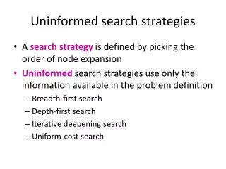
2. Uninformed search strategies • Uninformed (blind): • You have no clue whether one non-goal state is better than any other. Your search is blind. You don’t know if your current exploration is likely to be fruitful. • Various blind strategies: • Breadth-first search • Uniform-cost search • Depth-first search • Iterative deepening search (generally preferred) • Bidirectional search (preferred if applicable) • HILL-CLIMBINGSEARCH

3. Search strategy evaluation • A search strategy is defined by the order of node expansion • Strategies are evaluated along the following dimensions: • completeness: does it always find a solution if one exists? • time complexity: number of nodes generated • space complexity: maximum number of nodes in memory • optimality: does it always find a least-cost solution? • Time and space complexity are measured in terms of • b: maximum branching factor of the search tree • d: depth of the least-cost solution • m: maximum depth of the state space (may be ∞)

4. Uninformed search strategies • Queue for Frontier: • FIFO? LIFO? Priority? • Goal-Test: • When inserted into Frontier? When removed? • Tree Search or Graph Search: • Forget Explored nodes? Remember them?

5. Queue for Frontier • FIFO (First In, First Out) • Results in Breadth-First Search • LIFO (Last In, First Out) • Results in Depth-First Search • Priority Queue sorted by path cost so far • Results in Uniform Cost Search • Iterative Deepening Search uses Depth-First • Bidirectional Search can use either Breadth-First or Uniform Cost Search

6. When to do Goal-Test?When generated? When popped? • Do Goal-Test when node is popped from queue IF you care about finding the optimal path AND your search space may have both short expensive and long cheap paths to a goal. • Guard against a short expensive goal. • E.g., Uniform Cost search with variable step costs. • Otherwise, do Goal-Test when is node inserted. • E.g., Breadth-first Search, Depth-first Search, or Uniform Cost search when cost is a non-decreasing function of depth only (which is equivalent to Breadth-first Search). • REASON ABOUT your search space & problem. • How could I possibly find a non-optimal goal?

7. Repeated states • Failure to detect repeated states can turn a linear problem into an exponential one! • Test is often implemented as a hash table.

8. Solutions to Repeated States S B Graph search • Never explore a state explored before • Must keep track of all possible states (a lot of memory) • E.g., 8-puzzle problem, we have 9! = 362,880 states • Memory-efficient approximation for DFS/DLS • Avoid states on path to root: avoid looping paths. • Graph search optimality/completeness • Same as Tree search; just a space-time trade-off S B C C C S B S State Space Example of a Search Tree faster but memory inefficient

9. Breadth-first search • Expand shallowest unexpanded node • Frontier (or fringe): nodes in queue to be explored • Frontier is a first-in-first-out (FIFO) queue, i.e., new successors go at end of the queue. • Goal-Test when inserted. Future= green dotted circles Frontier=white nodes Expanded/active=gray nodes Forgotten/reclaimed= black nodes Initial state = A Is A a goal state? Put A at end of queue. frontier = [A]

10. Breadth-first search • Expand shallowest unexpanded node • Frontier is a FIFO queue, i.e., new successors go at end Expand A to B, C. Is B or C a goal state? Put B, C at end of queue. frontier = [B,C]

11. Breadth-first search • Expand shallowest unexpanded node • Frontier is a FIFO queue, i.e., new successors go at end Expand B to D, E Is D or E a goal state? Put D, E at end of queue frontier=[C,D,E]

12. Breadth-first search • Expand shallowest unexpanded node • Frontier is a FIFO queue, i.e., new successors go at end Expand C to F, G. Is F or G a goal state? Put F, G at end of queue. frontier = [D,E,F,G]

13. Breadth-first search • Expand shallowest unexpanded node • Frontier is a FIFO queue, i.e., new successors go at end Expand D to no children. Forget D. frontier = [E,F,G]

14. Breadth-first search • Expand shallowest unexpanded node • Frontier is a FIFO queue, i.e., new successors go at end Expand E to no children. Forget B,E. frontier = [F,G]

15. Example BFS

16. Properties of breadth-first search • Complete?Yes, it always reaches a goal (if b is finite) • Time?1+b+b2+b3+… + bd = O(bd) (this is the number of nodes we generate) • Space?O(bd) (keeps every node in memory, either in fringe or on a path to fringe). • Optimal? No, for general cost functions. Yes, if cost is a non-decreasing function only of depth. • With f(d) ≥ f(d-1), e.g., step-cost = constant: • All optimal goal nodes occur on the same level • Optimal goal nodes are always shallower than non-optimal goals • An optimal goal will be found before any non-optimal goal • Space is the bigger problem (more than time)

17. Uniform-cost search Breadth-first is only optimal if path cost is a non-decreasing function of depth, i.e., f(d) ≥ f(d-1); e.g., constant step cost, as in the 8-puzzle. Can we guarantee optimality for variable positive step costs ? (Why ? To avoid infinite paths w/ step costs 1, ½, ¼, …) Uniform-cost Search: Expand node with smallest path cost g(n). • Frontier is a priority queue, i.e., new successors are merged into the queue sorted by g(n). • Can remove successors already on queue w/higher g(n). • Saves memory, costs time; another space-time trade-off. • Goal-Test when node is popped off queue.

18. Uniform-cost search Uniform-cost Search: Expand node with smallest path cost g(n). Proof of Completeness: Given that every step will cost more than 0, and assuming a finite branching factor, there is a finite number of expansions required before the total path cost is equal to the path cost of the goal state. Hence, we will reach it. Proof of optimality given completeness: Assume UCS is not optimal. Then there must be an (optimal) goal state with path cost smaller than the found (suboptimal) goal state (invoking completeness). However, this is impossible because UCS would have expanded that node first by definition. Contradiction.

19. Uniform-cost search Implementation: Frontier = queue ordered by path cost. Equivalent to breadth-first if all step costs all equal. Complete? Yes, if b is finite and step cost ≥ ε > 0. (otherwise it can get stuck in infinite loops) Time? # of nodes with path cost ≤ cost of optimal solution. O(b1+C*/ε) ≈ O(bd+1) Space? # of nodes with path cost ≤ cost of optimal solution. O(b1+C*/ε) ≈ O(bd+1) Optimal? Yes, for any step cost ≥ ε > 0.

20. 6 1 A D F 1 3 2 4 8 S G B E 1 20 C The graph above shows the step-costs for different paths going from the start (S) to the goal (G). Use uniform cost search to find the optimal path to the goal. Exercise for at home

21. Depth-first search • Expand deepest unexpanded node • Frontier = Last In First Out (LIFO) queue, i.e., new successors go at the front of the queue. • Goal-Test when inserted. Future= green dotted circles Frontier=white nodes Expanded/active=gray nodes Forgotten/reclaimed= black nodes Initial state = A Is A a goal state? Put A at front of queue. frontier = [A]

22. Depth-first search • Expand deepest unexpanded node • Frontier = LIFO queue, i.e., put successors at front Expand A to B, C. Is B or C a goal state? Put B, C at front of queue. frontier = [B,C] Future= green dotted circles Frontier=white nodes Expanded/active=gray nodes Forgotten/reclaimed= black nodes Note: Can save a space factor of b by generating successors one at a time. See backtracking search in your book, p. 87 and Chapter 6.

23. Depth-first search • Expand deepest unexpanded node • Frontier = LIFO queue, i.e., put successors at front Expand B to D, E. Is D or E a goal state? Put D, E at front of queue. frontier = [D,E,C] Future= green dotted circles Frontier=white nodes Expanded/active=gray nodes Forgotten/reclaimed= black nodes

24. Depth-first search • Expand deepest unexpanded node • Frontier = LIFO queue, i.e., put successors at front Expand D to H, I. Is H or I a goal state? Put H, I at front of queue. frontier = [H,I,E,C] Future= green dotted circles Frontier=white nodes Expanded/active=gray nodes Forgotten/reclaimed= black nodes

25. Depth-first search • Expand deepest unexpanded node • Frontier = LIFO queue, i.e., put successors at front Future= green dotted circles Frontier=white nodes Expanded/active=gray nodes Forgotten/reclaimed= black nodes Expand H to no children. Forget H. frontier = [I,E,C]

26. Depth-first search • Expand deepest unexpanded node • Frontier = LIFO queue, i.e., put successors at front Expand I to no children. Forget D, I. frontier = [E,C] Future= green dotted circles Frontier=white nodes Expanded/active=gray nodes Forgotten/reclaimed= black nodes

27. Depth-first search • Expand deepest unexpanded node • Frontier = LIFO queue, i.e., put successors at front Expand E to J, K. Is J or K a goal state? Put J, K at front of queue. frontier = [J,K,C] Future= green dotted circles Frontier=white nodes Expanded/active=gray nodes Forgotten/reclaimed= black nodes

28. Depth-first search • Expand deepest unexpanded node • Frontier = LIFO queue, i.e., put successors at front Expand I to no children. Forget D, I. frontier = [E,C] Future= green dotted circles Frontier=white nodes Expanded/active=gray nodes Forgotten/reclaimed= black nodes

29. Depth-first search • Expand deepest unexpanded node • Frontier = LIFO queue, i.e., put successors at front Expand K to no children. Forget B, E, K. frontier = [C] Future= green dotted circles Frontier=white nodes Expanded/active=gray nodes Forgotten/reclaimed= black nodes

30. Depth-first search • Expand deepest unexpanded node • Frontier = LIFO queue, i.e., put successors at front Future= green dotted circles Frontier=white nodes Expanded/active=gray nodes Forgotten/reclaimed= black nodes Expand C to F, G. Is F or G a goal state? Put F, G at front of queue. frontier = [F,G]

31. Properties of depth-first search A • Complete? No: fails in loops/infinite-depth spaces • Can modify to avoid loops/repeated states along path • check if current nodes occurred before on path to root • Can use graph search (remember all nodes ever seen) • problem with graph search: space is exponential, not linear • Still fails in infinite-depth spaces (may miss goal entirely) • Time?O(bm) with m =maximum depth of space • Terrible if m is much larger than d • If solutions are dense, may be much faster than BFS • Space?O(bm), i.e., linear space! • Remember a single path + expanded unexplored nodes • Optimal? No: It may find a non-optimal goal first B C

32. Iterative deepening search • To avoid the infinite depth problem of DFS, only search until depth L, i.e., we don’t expand nodes beyond depth L.  Depth-Limited Search • What if solution is deeper than L?  Increase L iteratively.  Iterative Deepening Search • This inherits the memory advantage of Depth-first search • Better in terms of space complexity than Breadth-first search.

33. Iterative deepening search L=0

34. Iterative deepening search L=1

35. Iterative deepening search L=2

36. Iterative Deepening Search L=3

37. Iterative deepening search • Number of nodes generated in a depth-limited search to depth d with branching factor b: NDLS = b0 + b1 + b2 + … + bd-2 + bd-1 + bd • Number of nodes generated in an iterative deepening search to depth d with branching factor b: NIDS = (d+1)b0 + d b1 + (d-1)b2 + … + 3bd-2 +2bd-1 + 1bd = O(bd) • For b = 10, d = 5, • NDLS = 1 + 10 + 100 + 1,000 + 10,000 + 100,000 = 111,111 • NIDS = 6 + 50 + 400 + 3,000 + 20,000 + 100,000 = 123,450

38. Properties of iterative deepening search • Complete? Yes • Time?O(bd) • Space?O(bd) • Optimal? No, for general cost functions. Yes, if cost is a non-decreasing function only of depth.

39. Advantages of depth-first: Simple to implement; Needs relatively small memory for storing the state-space. Disadvantages of depth-first: Sometimes fail to find a solution (may be get stuck in an infinite long branch) -not complete; Notguaranteed to find an optimalsolution (may not find the shortest path solution); Can take a lot longer to find a solution. Advantages of breadth-first: Guaranteed to find a solution (if one exists) - complete; Depending on the problem, can be guaranteed to find an optimalsolution. Disadvantages of breadth-first: More complex to implement; Needs a lot of memory for storing the state space if the search space has a high branching factor. Depth-firstvs.Breadth-first

40. Bidirectional Search • Idea • simultaneously search forward from S and backwards from G • stop when both “meet in the middle” • need to keep track of the intersection of 2 open sets of nodes • What does searching backwards from G mean • need a way to specify the predecessors of G • this can be difficult, • e.g., predecessors of checkmate in chess? • which to take if there are multiple goal states? • where to start if there is only a goal test, no explicit list?

41. Bidirectional Search • Bidirectional search is a graph search algorithm that finds a shortest path from an initial vertex to a goal vertex in a directed graph. It runs two simultaneous searches: one forward from the initial state, and one backward from the goal, stopping when the two meet in the middle. The reason for this approach is that in many cases it is faster

42. The River Problem • Let’s consider the River Problem: A farmer wishes to carry a wolf, a duck and corn across a river, from the south to the north shore. The farmer is the proud owner of a small rowing boat called Bounty which he feels is easily up to the job. Unfortunately the boat is only large enough to carry at most the farmer and one other item. Worse again, if left unattended the wolf will eat the duck and the duck will eat the corn. How can the farmer safely transport the wolf, the duck and the corn to the opposite shore? River boat Farmer, Wolf, Duck and Corn

43. FWCD/- The River Problem • The River Problem: F=Farmer W=Wolf D=Duck C=Corn /=River How can the farmer safely transport the wolf, the duck and the corn to the opposite shore? -/FWCD

44. The River Problem • Problem formulation: • State representation: location of farmer and items in both sides of river [items in South shore / items in North shore] : (FWDC/-, FD/WC, C/FWD …) • Initial State: farmer, wolf, duck and corn in the south shore FWDC/- • Goal State: farmer, duck and corn in the north shore -/FWDC • Operators: the farmer takes in the boat at most one item from one side to the other side (F-Takes-W, F-Takes-D, F-Takes-C, F-Takes-Self [himself only]) • Path cost: the number of crossings

45. F D D F W D F-Takes-D F-Takes-S F-Takes-W W C F W C C F W D C WC/FD FWC/D C/FWD Initial State F-Takes-D F W C W C W F W D C F-Takes-S F-Takes-C F-Takes-D F D D F D C FD/WC D/FWC FDC/W Goal State The River Problem • Problem solution: (path Cost = 7) While there are other possibilities here is one 7 step solution to the river problem