Competitive Coevolution (Predator-Prey Coevolution)

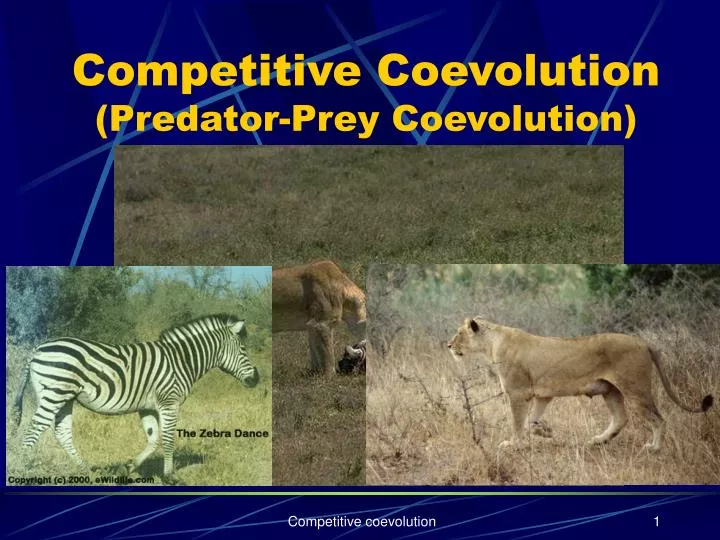
1. Competitive Coevolution(Predator-Prey Coevolution) Competitive coevolution

2. Coevolution • Simultaneous evolution of two or more species with coupled fitness. • Coevolving species either compete or cooperate. • Competitive coevolution: Fitness of individual based on direct competition with individuals of other species, which in turn evolve separately in their own populations (“prey-predator”). Competitive coevolution

3. Hillis 90 • Coevolving a population of sorting networks (candidate solutions) with a population of sorting problems (test-cases). • The fitness of a sorting network depends upon how good it solves sorting problems. • A sorting problem is scored according to how well it finds flaws in sorting networks. Competitive coevolution

4. Hillis 90 - Conclusions • Helps prevent large portions of the population from becoming stuck in local optima. • Testing becomes more efficient. Competitive coevolution

5. Paredis’life time fitness evaluation (LTFE) • First introduced by Paredis at 1994. • Replaces the “all-at-once” fitness calculation of a GA with a more partial but continuous fitness evaluation that occurs during the entire lifetime of an individual. • Allow both populations to coevolve. Competitive coevolution

6. LTFE (cont’d) • The fitness of a solution is defined as the number of test-cases satisfied by the solution during its last 20 encounters. • The fitness of a test-case is the number of times the test was violated by the 20 solutions it encountered most recently. • Hence, the test and solutions have an inverse fitness interaction (as in predator-prey systems). Competitive coevolution

7. LTFE pseudocode Competitive coevolution

8. LTFE Features • A few well-chosen test-cases provide sufficient information for solution’s evaluation. • The algorithm dynamically focuses on more difficult, not yet solved test-cases. Competitive coevolution

9. LTFE Examples • Coevolutionary neural net learning for classification. • Coevolutionary Constraint Satisfaction. • Symbiotic Coevolution. Competitive coevolution

10. Coevolutionary Neural Net Learning for Classification Find appropriate connection weights such that a neural net (NN) represents the correct mapping from [-1,1] x [-1,1] to a set of given classes {A,B,C,D} given 200 preclassified, randomly selected examples. Competitive coevolution

11. Coevolutionary Neural Net Learning for Classification Competitive coevolution

12. The Classification Process The input coordinates (x,y) are clamped on the assosiated input nodes of the neural net. Feed-forward propagation is executed. The result of the classification is the class corresponding to the output node with the highest activity level. The neural net is said to classify the example correctly when the output node associated with the correct class is the most active one. Competitive coevolution

13. Standard GA Versus CGA • The standard GA tests each newborn NN on all 200 training examples at once. • The fitness is defined as the number of training examples correctly classified by the NN. • In addition to the solution population the CGA has a test-cases population. This population contains the 200 preclassififed training examples. Competitive coevolution

14. Standard GA Versus CGA (cont’d) • The basic cycle of CGA is 3.75 times faster than that of the standard GA. • The standard GA was allowed to generate a total of 50,000 offspring. • The CGA was allowed to generate a total of 100,000 offspring. Competitive coevolution

15. Results Competitive coevolution

16. Discussion • The computational demand of the CGA is considerably smaller than that of the traditional GA. • The CGA clearly beats the standard GA in terms of solution quality. Competitive coevolution

17. Discussion (cont’d) Reasons for the considerable performance increase: • Once an NN is considered potentially good it is put under closer scrutiny. • Coevolution forces the CGA to focus on not yet solved examples. The latter can be easily observed in the classification task: only the examples that are situated near the boundaries between different classes have a high fitness value. Competitive coevolution

18. Discussion (cont’d) Competitive coevolution

19. Constraint Satisfaction Problems (CSP) • Instance: • a set of n variables {xi}, each has an associated domain, Di, of possible values. • A set C of constraints that describe relations between the values of the xi (e.g., x1 x3). • A valid solution consists of an assignment of values to the xi such that all constraints in C are satisfied. Competitive coevolution

20. The N-Queens Problem • Placing n queens on a n x n chess board so that no two queens attack each other. • Representation: n variables xi, each such variable represents one column on the chess board (e.g., x2=3 indicates that a queen is positioned in the third row of the second column). • Constraints: • Row-constraint: xixji j • Diagonal-constraint: |xi – xj|  |i – j|  i j Competitive coevolution

21. CGA • Solution population consists of n-dimensional vectors containing integers between 1 and n. • The 2n constraints constitute the test-population. • An inverse fitness interaction.. • Fit solutions and constrains are more likely to be involved in an encounter (e.g., diagonal constraints). Competitive coevolution

22. GA, CGA-, and CGA • GA uses only a population of solutions. • CGA- is identical to CGA, except the constraints do not have any fitness (LTFE without coevolution). • CGA. All three algorithms were tested with 50-queens problem, a solution population of size 250, and were allowed to generate a total of 200,000 offspring. Competitive coevolution

23. Results (10 runs) • GA never found a global solution satisfying all constraints (average of 95.7/100 constraints satisfied). • CGA- found such a solution only once (average: 97.2). • CGA was successful seven times (average: 99.4). Competitive coevolution

24. Conclusion It is the combination of LTFE and coevolution that boosts the power of a CGA. Either one of these mechanisms alone yields clearly inferior results. Competitive coevolution

25. Symbiotic Coevolution Competitive coevolution

26. Symbiotic Coevolution with CGA • Investigation of the symbiotic evolution of solutions and their genetic representation (i.e., the ordering of the genes). • It is hard to choose a good genetic representation: • One might not know the epistatic interactions in advance. • One linear ordering might not be sufficient to express all epistatic interactions. Competitive coevolution

27. Symbiotic Coevolution with CGA (cont’d) • Using symbiotic (cooperative) coevoultion to obtain tight interactions between solutions and representations. • Success one one side improves the chances of survival of the other. • A representation adapted to the solutions currently in the population speeds up the search for even better solutions that in their turn might progress optimally when yet another representation is used. • SYMBIOT. Competitive coevolution

28. The Test Problems Given a matrix A (of size n x n), and an n-dimensional vector b solve the equation Ax = b. Competitive coevolution

29. The Test Problems (espistasis ) • The diagonal elements of A are randomly chosen from the set {1,2,…,9}. • When all off-diagonal elements of A are zero then the problem is not epistatic. • By setting off-diagonal entries to non-zero, the degree of espistasis is increased. • Due to transitivity, the degree of epistisis can be gradually increased by setting elements immediately above the diagonal to non-zero. Competitive coevolution

30. The Test Problems (cont’d) • bi are chosen such that all components xi are equal to 1. • n =10. That is, A is a 10 x 10 matrix, b,x are of size 10. • The performance of a standard GA critically depends on the representation used. • The choice of representation is irrelevant only in the two extreme cases. • The main problem: a standard GA uses only one, a priori defined representation. Competitive coevolution

31. SYMBIOT • A permutation (ordering) population coevolves alongside a population of candidate solutions. • Each member of the solutions population is represented as a real-numbers 10-dimensional vector that uses the same a priori chosen representation (<x1,…,xn>). • A permutation is a 10-dimensional vector that describes a reordering of solution genes. • The permutation constructs the representation operated on by recombination. Competitive coevolution

32. Basic Cycle of SYMBIOT * * Fitness values of the solutions are negative Competitive coevolution

33. Example • sol1 = < x1, x2, x3, x4> sol2 = < y1, y2, y3, y4> perm = <4,1,3,2>. • perm(sol1) = < x4, x1, x3, x2> perm(sol2) = < y4, y1, y3, y2>. • p-sol-child = mutate-crossover(sol1,sol2) = < x4, x1 , y3, y2>. • sol-child = inv-perm(p-sol-child) = < x1, y2, y3, x4>. Competitive coevolution

34. SYMBIOT (cont’d) • A good permutation puts the relevant functionally correlated genes near each other. • LTFE takes care of noise in evaluating a permutation. • Only permutations undergoes LTFE. Competitive coevolution

35. FIXED and RAND • FIXED uses the best possible fixed representation. • SYMBIOT not only has to solve the set of equations; it has to solve the representation problem as well. • RAND generates for each couple of parents a random permutation: Competitive coevolution

36. Experimental Setup • Solution population’s size = 1000. • Permutation population’s size = 100. • All results averaged over 10 runs. Two series of experiments are reported: • SYMBIOT versus FIXED and RAND for problems with different degrees of epistisis. • The grouping of functionally related genes in SYMBIOT. Competitive coevolution

37. The Test Problems • Trivial – no epistisis. • Simple – set of linkage {(xi-1,xi)}even(i), this is done by assigning Ai-1,i random values between 1 and 9 for even i’s. (non-overlapping linkage). • MEDIUM – {(x1,x2), (x2,x3), (x3,x4), (x4,x5), (x5,x6), (x7,x8), (x9,x10)}. • COMPLEX – {(x1,x2), (x2,x3), (x3,x4), (x4,x5), (x5,x6), (x6,x7), (x7,x8), (x8,x9), (x9,x10)}. Competitive coevolution

38. Results Competitive coevolution

39. SYMBIOT’s Grouping of Related Genes • Defining length of a given permutation and a given pair of genes, is how far apart the permutation puts these genes. • Average defining length of a set of pairs of genes is the average defining length for each pair of genes in the set and for each member of the permutation population. Competitive coevolution

40. Grouping of Genes when solving “SIMPLE” Competitive coevolution

41. Discussion • SYMBIOT clearly exhibits a clear selective pressure toward grouping related variables and leaving unrelated genes apart. • Q: Why does the average defining length of the linked variables gradually increase after its initial drop? • A: At the later stages of a run, all solutions get more and more similar. As a result, the selective pressure to group particular genes decreases. Competitive coevolution

42. The “5-5” Problem • One linkage away from total epistisis (x5,x6). • The variables x1, x2, x3, x4, x5 are completely interlinked. The same is true for the other 5 variables. • In the results “related” now gives the average defining length of the shortest schema containing x1, x2, x3, x4, x5 and of the shortest schema containing x6, x7, x8, x9, x10. Competitive coevolution

43. Grouping of Genes when solving “5-5” Competitive coevolution

44. Discussion • Similar observations as the “SIMPLE” experiment. • The curve is less smooth than the “SIMPLE” experiment due to the high level of epistisis. • The effects of using different recombination operators. Competitive coevolution