Download
1 / 46
460 likes | 707 Views
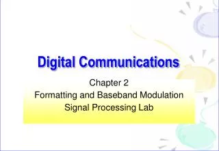
Digital Communications. Engr Ghulam Shabbir. Quantization Process.

E N D
Digital Communications Engr Ghulam Shabbir
Quantization Process • A continuous signal , such as voice , has a continuous range of amplitude and therefore its samples have a continuous amplitude range. In other words, within the finite amplitude range of signals, we find an infinite number of amplitude levels. • The original continuous signal is approximated by a signal constructed of discrete amplitudes selected on a minimum error basis from the available set. • The existence of a finite number of discrete amplitude levels is a basic condition of pulse code modulation. • Amplitude quantization is defined as process of transforming the sample amplitude m(nTs) of a message signal m(t) at time t = nTinto a discrete amplitude v(nTs) taken from a finite set of possible amplitudes.
Quantization Process • Being the process in the quantizer as memoryless and continuous , sample is considered as a scalar quantity m instead of m(nTs) as shown the diagram of the quantizer. • The signal amplitude m id specified by the index k if it lies inside the partition cell.
Quantizer can be: • Uniform Quantizer • Non-uniform Quantizer • In a uniform quantizer, the representation levels are uniformly spaced; otherwise, the quantizer is nonuniform. • The quantizer characteristic can also be of midtread or midrise type. • Below Fig a shows the input-output characteristic of a uniform quantizer of the midtread type, which is so called because the origin lies in the middle of a tread of the staircaselike graph. • Fig b shows the corresponding input-output characteristics of a uniform quantizer of the midrise type, in which the origin lies in the middle of a rising part of the staircaselike graph. • Note that both the midtread and midrise types of uniform quantizers illustrated in the fig are symmetric about the origin.
Figure 3.10 Two types of quantization: (a) midtread and (b) midrise. 13
The use of quantization introduces an error defined as the difference between the input signal m and the output signal v. The error is called quantization noise. • Below Fig illustrates a typical variation of the quantization noise as a function of time, assuming the use of a uniform quantizer of the midtread type.
Quantization Noise Figure 3.11 Illustration of the quantization process. (Adapted from Bennett, 1948, with permission of AT&T.) 14
- Am 0 Am
Pulse Code Modulation • Following are the various operations that constitute a basic PCM system: • Sampling • Quantization • Encoding • Regeneration • Decoding • Filtering
Pulse Code Modulation Figure 3.13 The basic elements of a PCM system.
Quantization • The quantization process may follow a uniform law.
Line codes: 1. Unipolar nonreturn-to-zero (NRZ) Signaling 2. Polar nonreturn-to-zero(NRZ) Signaling 3. Unipor nonreturn-to-zero (RZ) Signaling 4. Bipolar nonreturn-to-zero (BRZ) Signaling 5. Split-phase (Manchester code)
Figure 3.15 Line codes for the electrical representations of binary data. (a) Unipolar NRZ signaling. (b) Polar NRZ signaling. (c) Unipolar RZ signaling. (d) Bipolar RZ signaling. (e) Split-phase or Manchester code.
Differential Encoding (encode information in terms of signal transition; a transition is used to designate Symbol 0) Regeneration (reamplification, retiming, reshaping ) Two measure factors: bit error rate (BER) and jitter. Decoding and Filtering
3.8 Noise consideration in PCM systems (Channel noise, quantization noise) (will be discussed in Chapter 4)
Time-Division Multiplexing Synchronization Figure 3.19 Block diagram of TDM system.
3.11 Virtues, Limitations and Modifications of PCM Advantages of PCM 1. Robustness to noise and interference 2. Efficient regeneration 3. Efficient SNR and bandwidth trade-off 4. Uniform format 5. Ease add and drop 6. Secure
The modulator consists of a comparator, a quantizer, and an accumulator The output of the accumulator is Two types of quantization errors : Slope overload distortion and granular noise
Slope Overload Distortion and Granular Noise ( differentiator )
Delta-Sigma modulation (sigma-delta modulation) The modulation which has an integrator can relieve the draw back of delta modulation (differentiator) Beneficial effects of using integrator: 1. Pre-emphasize the low-frequency content 2. Increase correlation between adjacent samples (reduce the variance of the error signal at the quantizer input ) 3. Simplify receiver design Because the transmitter has an integrator , the receiver consists simply of a low-pass filter. (The differentiator in the conventional DM receiver is cancelled by the integrator )
Figure 3.25 Two equivalent versions of delta-sigma modulation system.
3.13 Linear Prediction (to reduce the sampling rate) Consider a finite-duration impulse response (FIR) discrete-time filter which consists of three blocks : 1. Set of p ( p: prediction order) unit-delay elements (z-1) 2. Set of multipliers with coefficients w1,w2,…wp 3. Set of adders ( )
For convenience, we may rewrite the Wiener-Hopf equations The filter coefficients are uniquely determined by
Linear adaptive prediction (If for varying k is not available)
Differentiating (3.63), we have Substituting (3.71) into (3.69)
Figure 3.27 Block diagram illustrating the linear adaptive prediction process.
3.14 Differential Pulse-Code Modulation (DPCM) Usually PCM has the sampling rate higher than the Nyquist rate .The encode signal contains redundant information. DPCM can efficiently remove this redundancy. Figure 3.28 DPCM system. (a) Transmitter. (b) Receiver.
From (3.74) Input signal to the quantizer is defined by:
3.15 Adaptive Differential Pulse-Code Modulation (ADPCM) Need for coding speech at low bit rates , we have two aims in mind: 1. Remove redundancies from the speech signal as far as possible. 2. Assign the available bits in a perceptually efficient manner. Figure 3.29 Adaptive quantization with backward estimation (AQB). Figure 3.30 Adaptive prediction with backward estimation (APB).