Download

1 / 36
370 likes | 945 Views
Noun Phrase Extraction. A Description of Current Techniques. What is a noun phrase?. A phrase whose head is a noun or pronoun optionally accompanied by a set of modifiers Determiners: Articles: a, an, the Demonstratives: this, that, those Numerals: one, two, three

E N D
Noun Phrase Extraction A Description of Current Techniques
What is a noun phrase? • A phrase whose head is a noun or pronoun optionally accompanied by a set of modifiers • Determiners: • Articles: a, an, the • Demonstratives: this, that, those • Numerals: one, two, three • Possessives: my, their, whose • Quantifiers: some, many • Adjectives: the red ball • Relative clauses: the books that I bought yesterday • Prepositional phrases: the man with the black hat
Is that really what we want? • POS tagging already identifies pronouns and nouns by themselves • The man whose red hat I borrowed yesterday in the street that is next to my house lives next door. • [The man[whose red hat [I borrowed yesterday]RC ]RC[in the street]PP[that is next to my house]RC]NP lives [next door]NP. • Base Noun Phrases • [The man]NP whose [red hat]NP I borrowed [yesterday ]NP in [the street]NP that is next to [my house]NP lives [next door]NP.
How Prevalent is this Problem? • Established by Steven Abney in 1991 as a core step in Natural Language Processing • Quite explored
What were the successful early solutions? • Simple Rule-based/ Finite State Automata Both of these rely on the aptitude of the linguist formulating the rule set.
Simple Rule-based/ Finite State Automata • A list of grammar rules and relationships are established. For example: • If I have an article preceding a noun, that article marks the beginning of a noun phrase. • I cannot have a noun phrase beginning after an article • The simplest method
FSA simple NPE example noun/ pronoun/ determiner determiner/adjective noun/ pronoun S0 S1 NP adjective Relative clause/ Prepositional phrase/ noun
Simple rule NPE example • “Contextualization” and “lexicalization” • Ratio between the number of occurrences of a POS tag in a chunk and the number of occurrences of this POS tag in the training corpora
Parsing FSA’s, grammars, regular expressions: LR(k) Parsing • The L means we do Left to right scan of input tokens • The R means we are guided by Rightmost derivations • The k means we will look at the next k tokens to help us make decisions about handles • We shift input tokens onto a stack and then reduce that stack by replacing RHS handles with LHS non-terminals
An Expression Grammar • E -> E + T • E -> E - T • E -> T • T -> T * F • T -> T / F • T -> F • F -> (E) • F -> i
An LR(1) NPE Example Stack Input Action [] N V N SH N [N] V N RE3.) NP N [NP] V N SH V [NP V] N SH N [NP V N] RE3.) NP N [NP V NP] RE4.) VP V NP [NP VP] RE1.) S NP VP [S] Accept! • S NP VP • NP Det N • NP N • VP V NP (Abney, 1991)
Why isn’t this enough? • Unanticipated rules • Difficulty finding non-recursive, base NP’s • Structural ambiguity
Structural Ambiguity “I saw the man with the telescope.” S S NP VP NP VP V VP I NP I NP saw V N N DET PP DET PP saw the man the man PRP DET N PRP DET N telescope with the telescope with the
What are the more current solutions? • Machine Learning • Transformation-based Learning • Memory-based Learning • Maximum Entropy Model • Hidden Markov Model • Conditional Random Field • Support Vector Machines
Machine Learning means TRAINING! • Corpus: a large, structured set of texts • Establish usage statistics • Learn linguistics rules • The Brown Corpus • American English, roughly 1 million words • Tagged with the parts of speech • http://www.edict.com.hk/concordance/WWWConcappE.htm
Transformation-based Machine Learning • An ‘error-driven’ approach for learning an ordered set of rules • 1. Generate all rules that correct at least one error. • 2. For each rule: (a) Apply to a copy of the most recent state of the training set. (b) Score the result using the objective function. • 3. Select the rule with the best score. • 4. Update the training set by applying the selected rule. • 5. Stop if the score is smaller than some pre-set threshold T; otherwise repeat from step 1.
Transformation-based NPE example • Input: • “WhitneyNN currentlyADV hasVB theDT rightADJ ideaNN.” • Expected output: • “[NP Whitney] [ADV currently] [VB has] [NP the right idea].” • Rules generated (all not shown): FromToIf NN NP always ADJ NP the previous word was ART DT NP the next word is an ADJ DT NP the previous word was VB
Memory-based Machine Learning • Classify data according to similarities to other data observed earlier • “Nearest neighbor” • Learning • Store all “rules” in memory • Classification: • Given new test instance X, • Compare it to all memory instances • Compute a distance between X and memory instance Y • Update the top k of closest instances (nearest neighbors) • When done, take the majority class of the k nearest neighbors as the class of X Daelemans, 2005
Memory-based Machine Learning Continued • Distance…? • The Overlapping Function: Count the number of mismatching features • The Modified Value Distance Metric (MVDM) Function: estimate a numeric distance between two “rules” • The distance between two N-dimensional vectors A, B with discrete (for example symbolic) elements, in a K class problem, is computed using conditional probabilities: • d(A,B) = Σj..nΣi..k (P(Ci I Aj) - P(Ci | Pj)) • where p(CilAj) is estimated by calculating the number Ni(Aj) of times feature Ajoccurred in vectors belonging to class Ci, and dividing it by the number of times feature Ajoccurred for any class Dusch, 1998
Memory-based NPE example • Suppose we have the following candidate sequence: • DT ADJ ADJ NN NN • “The beautiful, intelligent summer intern” • In our rule set we have: • DT ADJ ADJ NN NNP • DT ADJ NN NN
Maximum Entropy • The least biased probability distribution that encodes information maximizes the information entropy, that is, the measure of uncertainty associated with a random variable. • Consider that we have m unique propositions • The most informative distribution is one in which we know one of the propositions is true – information entropy is 0 • The least informative distribution is one in which there is no reason to favor any one proposition over another – information entropy is log m
Maximum Entropy applied to NPE • Let’s consider several French translations of the English word “in” • p(dans) + p(en) + p(á) + p(au cours de) + p(pendant) = 1 • Now suppose that we find that either dans or en is chosen 30% of the time. We must add that constraint to the model and choose the most uniform distribution • p(dans) = 3/20 • p(en) = 3/20 • p(á) = 7/30 • p(au cours de) = 7/30 • p(pendant) = 7/30 • What if we now find that either dans or áis used half of the time? • p(dans) + p(en) = .3 • p(dans) + p(á) = .5 • Now what is the most “uniform” distribution? Berger, 1996
Hidden Markov Model • In a statistical model of a system possessing the Markov property… • There are a discrete number of possible states • The probability distribution of future states depends only on the present state and is independent of past states • These states are not directly observable in a hidden Markov model. • The goal is to determine the hidden properties from the observable ones.
Hidden Markov Model • a: transition probabilities • x: hidden states • y: observable states • b: output probabilities
HMM Example • states = ('Rainy', 'Sunny') • observations = ('walk', 'shop', 'clean') • start_probability = {'Rainy': 0.6, 'Sunny': 0.4} • transition_probability = { 'Rainy' : {'Rainy': 0.7, 'Sunny': 0.3}, 'Sunny' : {'Rainy': 0.4, 'Sunny': 0.6}, } • emission_probability = { 'Rainy' : {'walk': 0.1, 'shop': 0.4, 'clean': 0.5}, 'Sunny' : {'walk': 0.6, 'shop': 0.3, 'clean': 0.1}, } In this case, the weather possesses the Markov property
HMM as applied to NPE • In the case of noun phrase extraction, the hidden property is the unknown grammar “rule” • Our observations are formed by our training data • Contextual probabilities represent the transition states • that is, given our previous two transitions, what is the likelihood of continuing, ending, or beginning a noun phrase/ P(oi|oj-1,oj-2) • Output probabilities • Given our current state transition, what is the likelihood of our current word being part of, beginning, or ending a noun phrase/ P(ij|oj) • MaxO1…OT( πj:1…T P(oi|oj-1,oj-2) · P(ij|oj) )
The Viterbi Algorithm • Now that we’ve constructed this probabilistic representation, we need to traverse it • Finds the most likely sequence of states
Viterbi Algorithm Whitney gave a painfully long presentation. B I O
Conditional Random Fields • An undirected graphical model in which each vertex represents a random variable whose distribution is to be inferred, and each edge represents a dependency between two random variables. In a CRF, the distribution of each discrete random variable Y in the graph is conditioned on an input sequence X Yi could be B,I,O in the NPE case … y1 y2 y4 yn y3 yn-1 x1,…, xn-1, xn
Conditional Random Fields • The primary advantage of CRF’s over hidden Markov models is their conditional nature, resulting in the relaxation of the independence assumptions required by HMM’s • The transition probabilities of the HMM have been transformed into feature functions that are conditional upon the input sequence
Support Vector Machines • We wish to graph an number of data points of dimension p and separate those points with a p-1 dimensional hyperplane that guarantees the maximum distance between the two classes of points – this ensures the most generalization • These data points represent pattern samples whose dimension is dependent upon the number of features used to describe them • http://www.csie.ntu.edu.tw/~cjlin/libsvm/#GUI
What if our points are separated by a nonlinear barrier? • The Kernel function (Φ): maps points from 2d to 3d space • The Radial Basis Function is the best function that we have for this right now
SVM’s applied to NPE • Normally, SVM’s are binary classifiers • For NPE we generally want to know about (at least) three classes: • B: a token is at the beginning of a chunk • I: a token is inside a chunk • O: a token is outside a chunk • We can consider one class vs. all other classes for all possible combinations • We could do a pairwise classification • If we have k classes, we build k · (k-1)/2 classifiers
Performance Metrics Used • Precision = number of correct responses number of responses • Recall = number of correct responses number correct in key • F-measure = (β2 + 1) RP (β2R)+ P Where β2 represents the relative weight of recall to precision (typically 1) (Bikel, 1998)