Spatial Filtering

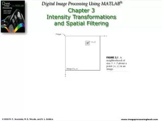
Spatial Filtering CS474/674 - Prof. Bebis Sections 3.4, 3.5, 3.6, 3.7, 3.8

output image Spatial Filtering Methods

Spatial Filtering (cont’d) • The word “filtering” comes from the frequency domain where “filters” are classified as: • Low-pass (i.e., preserve low frequencies) • High-pass (i.e., preserve high frequencies) • Band-pass (i.e., preserve frequencies within a band) • Band-reject (i.e., reject frequencies within a band)

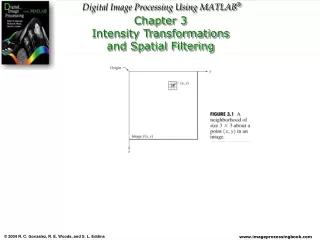
output image Spatial Filtering (cont’d) • Need to define: (1) a neighborhood (or mask) (2) an operation

Spatial Filtering – Neighborhood (or Mask) • Typically, the neighborhood is rectangular and its size is much smaller than that of f(x,y) - e.g., 3x3 or 5x5

output image Spatial filtering - Operation • Manipulate the pixel values, e.g., z’5 = 5z1 -3z2+z3-z4-2z5-3z6+z8-z9-9z7 z’5 = max(z1,z2,z3,z4,z5,z6,z7,z8,z9)

output image Linear vs Non-Linear filters • A filter is called linear when its output is a linear combination of the inputs, e.g., z’5 = 5z1 -3z2+z3-z4-2z5-3z6+z8-z9-9z7

output image Linear vs Non-Linear filters (cont’d) • A filter is called non-linearwhen its output is not a linear combination of the inputs, e.g., z’5 = max(z1,z2,z3,z4,z5,z6,z7,z8,z9)

output image Correlation (linear operator) • The output of correlation is a weighted sum of input pixels. Need to define mask weights!

w(i,j) Filtered Image f(i,j) Correlation (cont’d) g(i,j) Filtered image is generated by moving the center of the mask at every location of the input image.

Handling Pixels Close to Boundaries pad with zeroes 0 0 0 ……………………….0 0 0 0 ……………………….0

Correlation (cont’d) Often used in applications where we need to measure the similarity between images or parts of images (e.g., template matching).

Convolution (linear operator) • Similar to correlation except that the mask is first flipped both horizontally and vertically. • If w(i, j) is symmetric (i.e., w(i, j)=w(-i,-j)),then convolution is equivalent to correlation!

Example Correlation: Convolution:

Filter Categories • We will focus on two types of filters: • Smoothing (low-pass) filters • Sharpening (high-pass) filters

Smoothing Filters (low-pass) • Useful for reducing noise and eliminatingsmall details. • The elements of the mask must be positive. • Mask elements sum to 1 (assuming normalization).

Smoothing filters – Example input image smoothed image

Sharpening Filters (high-pass) • Useful for highlighting fine details. • The elements of the mask contain both positive and negative weights. • Mask elements sum to 0.

Sharpening Filters - Example • Useful for highlighting fine details. • e.g., emphasize edges

Sharpening Filters - Example input image sharpened image (for better visualization, the original image has been added to the sharpened image)

Common Smoothing Filters • Averaging • Gaussian • Median filtering (non-linear)

Smoothing Filters: Averaging

Smoothing Filters: Averaging (cont’d) • Mask size determines degree of smoothing (i.e., loss of detail). original 3x3 5x5 7x7 15x15 25x25

Smoothing Filters: Averaging (cont’d) Example: extract largest, brightest objects 15 x 15 averaging image thresholding

Smoothing filters: Gaussian • The weights are samples of a 2D Gaussian function:

Smoothing filters: Gaussian (cont’d) • Mask size depends on σ

Smoothing filters: Gaussian (cont’d) • σ controls the amount of smoothing σ = 3 σ = 1.4

Smoothing filters: Gaussian (cont’d)

Averaging vs Gaussian Smoothing Averaging Gaussian

Smoothing Filters: Median Filtering(non-linear) • Very effective for removing “salt and pepper” noise (i.e., random occurrences of black and white pixels). median filtering averaging

Smoothing Filters: Median Filtering (cont’d) • Replace each pixel by the median in a neighborhood around the pixel. • The size of the neighborhood controls the amount of smoothing.

Common Sharpening Filters • Unsharp masking • High Boost filter • Gradient (1st derivative) • Laplacian (2nd derivative)

Sharpening Filters: Unsharp Masking • Obtain a sharp image by subtracting a lowpass filtered (i.e., smoothed) image from the original image: - = (with contrast enhancement)

Sharpening Filters: High Boost • Image sharpening emphasizes edges but details are lost. • Idea: amplify input image, then subtract a lowpass image. (A-1) + =

Sharpening Filters: High Boost (cont’d) • If A=1, the result is unsharp masking. • If A>1, part of the original image is added back to the high pass filtered image. High boost One way to implement high boost filtering is using the masks below

Sharpening Filters: High Boost (cont’d) A=1.9 A=1.4

Sharpening Filters: Derivatives • The derivative of an image results in a sharpened image. • Image derivatives can be computed using the gradient:

Gradient • The gradient is a vector which has magnitude and direction: (approximation) or

Gradient (cont’d) • Gradient magnitude: provides information about edge strength. • Gradient direction:perpendicular to the direction of the edge.

Δx Gradient Computation • Approximate partial derivatives using finite differences:

Gradient Computation (cont’d) f(x3,y3)-f(x3,y2) sensitive to horizontal edges y3-y2 y2=y3+Dy, y3=y, x3=x, Dy=1 sensitive to vertical edges

Example: visualize partial derivatives

Implement Gradient Using Masks • We can implement and using masks: (x+1/2,y) good approximation at (x+1/2,y) (x,y+1/2) * * good approximation at (x,y+1/2)

Implement Gradient Using Masks (cont’d) • A different approximation of the gradient: good approximation (x+1/2,y+1/2) * • We can implement and using the following masks:

Implement Gradient Using Masks (cont’d) • Other approximations Prewitt Sobel

Example: Gradient Magnitude Image Gradient Magnitude (isotropic)

Laplacian The Laplacian (2nd derivative) is defined as: (dot product) Approximate 2nd derivatives:

Laplacian (cont’d) Laplacian Mask output image input image Edges can be found by detecting the zero-crossings 5 5 5 5 -5 -10 -5 -10 5 10 -10

Example: Laplacian vs Gradient Sobel Laplacian • Laplacian localizes edges better (zero-crossings). • Higher order derivatives more sensitive to noise. • Laplacian is less computational expensive. • Laplacian can provide edge magnitude information • but no information about edge direction.

Quiz 2 • When: Monday, September 30th • What: Spatial Filtering

Spatial Filtering