Download
1 / 21
210 likes | 213 Views
Initial Application of the Adaptive Grid Air Quality Model. Dr. M. Talat Odman, Maudood N. Khan Georgia Institute of Technology Dr. Ravi Srivastava United States Environmental Protection Agency Dr. D. Scott McRae North Carolina State University. Motivation.

E N D
Initial Application of the Adaptive Grid Air Quality Model Dr. M. Talat Odman, Maudood N. Khan Georgia Institute of Technology Dr. Ravi Srivastava United States Environmental Protection Agency Dr. D. Scott McRae North Carolina State University Georgia Institute of Technology
Motivation • Inadequate grid resolution necessitated by computational limitations is an important source of uncertainty in air quality models (AQMs). • Fixed grids (nested and multiscale) have limitations: • Assumptions are made in placing finer grid resolution, • Some accuracy is lost due to grid interface problems, • Fixed grids cannot adjust to dynamic changes in solution requirements. • Adaptive grids offer an effective and potentially more efficient alternative. • Interactions of urban and point source plumes with the surrounding atmosphere can be better resolved. Georgia Institute of Technology
Adaptive Grid Methodology • The number of grid nodes is constant • The domain is divided into NxM quadrilateral grid cells • Grid node movement criteria • A user defined function (weight function) controls the grid node movement. Defines the grid resolution requirements • Grid nodes move throughout the simulation • Grid cells are automatically refined/coarsened to reduce error in variables • The structure of the grid is maintained Georgia Institute of Technology
Snapshot of the Adaptive Grid from the Tennessee Valley Simulation Georgia Institute of Technology
Adaptive Grid ModelingTwo consecutive steps • Adaptation step: Freeze the concentration field and move the grid nodes • Grid Adaption step • Weight function computation • Grid node repositioning • Concentration redistribution • Solution preparation step • Meteorological data processing • Emissions data processing • Coordinate transformation • Solution Step: Freeze the grid nodes and advance the concentration field in time Georgia Institute of Technology
Grid Adaption Step:Weight Function • The weight function can be built as a linear combination of errors in different species: • the Laplacian operator (curvature) represents the error in species concentration • So far in our ozone simulations, we used the curvature in surface layer NO concentrations only. • We are investigating other combinations. Georgia Institute of Technology
4 3 i 1 2 Grid Adaption Step:Grid Movement • The new position of grid node i is calculated by a center-of-mass scheme: • where are the original positions (i.e., before movement) of the centroids of four cells that share grid node i • are the values of the weight function at those locations. Georgia Institute of Technology
Grid Adaption Step:Redistribution of Concentrations • After repositioning of the grid nodes, concentration values must be assigned to the new grid locations. • Holding the concentration fields fixed and moving the grid is equivalent to advection on a fixed grid. • We use a high-order accurate and monotonic advection scheme for interpolation (Piecewise parabolic method of Collela and Woodward, 1984). • If the maximum of all grid-node movements is below a preset tolerance, the grid is considered to have converged. • Otherwise, the process (i.e., calculation of the weight function, movement of grid nodes and interpolation of concentration values to new grid locations) is reiterated. Georgia Institute of Technology
Solution preparation step:Processing of Meteorological Inputs • Meteorological inputs must be mapped onto the “adapted” grid, in preparation for the solution step. • The ideal solution would be to run a meteorological model (MM), which can operate on the same adaptive grid, in parallel with the AQM. • Currently, such a model does not exist. • We are using hourly data from a very high-resolution fixed grid MM and interpolating the necessary inputs (e.g., temperature, wind and humidity fields) to the adapted grid locations. Georgia Institute of Technology
Solution preparation step:Processing of Emissions • Emission inputs must also be mapped onto the “adapted” grid. • We treat all emission sources as either point or area. • We currently lump the mobile sources into the area-source category. • For point sources, the grid cell containing the location of each stack is identified using efficient search algorithms. • Area source emissions are first mapped onto a high-resolution fixed grid referred to as the “emission” grid • The intersection of this “emission” grid with each adaptive grid is calculated. Georgia Institute of Technology
Solution preparation step:Area Source Emissions • The mass emitted into the adaptive grid cell is the sum of the products of the intersection area with the emission flux of . Georgia Institute of Technology
Solution preparation step:Coordinate Transformation • The non-uniform “adapted” grid in the horizontal (x,y) plane can be transformed into a uniform grid in the (x,h) plane: • The metrics of the transformation are: • These are calculated numerically. Georgia Institute of Technology
Solution Step • Atmospheric diffusion equations in (x,h,s) space can be written as: • where J is the Jacobian of the transformation Georgia Institute of Technology
Solution Step (Continued) • The components of the wind vector in x and h directions are: • Similar relations exist for other “contravariant” quantities. • Solution algorithms developed for uniform grids can now be used in the (x,h,s) space. Georgia Institute of Technology
Model Verification: Ozone Simulation in Tennessee Valley • We are verifying the adaptive grid model by simulating ozone air quality in the Tennessee Valley for the July 7-17, 1995 period. • Meteorological inputs are provided by the Regional Atmospheric Modeling System (RAMS) at 4x4 km resolution. • The Southern Appalachian Mountains Initiative (SAMI) emissions inventory is used. • There are over 9000 point sources in the domain including some of the largest power plants in the U.S.A. • Area sources are mapped onto a 4x4 km emissions grid. Georgia Institute of Technology
Model Verification (Continued) • The adaptive AQM grid consists of 112 by 65 cells, initially at 8x8 km resolution. The cell-size may drop to few hundred meters during the simulation. • In the vertical, there are 20 unequally spaced layers extending from the surface to 5340 m. • The grid is adapted once an hour to surface layer NO concentrations. The grid structure is the same for all vertical layers. • Two fixed gridAQM simulations at 4x4 and 8x8-km resolution have been performed Georgia Institute of Technology
NO levels (ppm): 11:00 EST July 9, 1995 Fixed Grid 8x8km Adaptive Grid Georgia Institute of Technology
O3 levels (ppm): 12:00 EST July 9, 1995 Fixed Grid 8x8km Adaptive Grid Georgia Institute of Technology
Conclusion • We developed an adaptive grid AQM. • A simulation with this model can be viewed as a sequence of two consecutive steps: • Adaptation step: the grid nodes move while the concentration fields remain unchanged • Solution step: the grid nodes remain fixed while the concentration fields are advanced in time • For verification, the model was compared to a fixed grid AQM with the same number of grid cells: • Adaptive AQM showed more detail in NO gradients • Adaptive AQM estimated higher ozone peaks • An evaluation using observed data is under way. Georgia Institute of Technology