3.8.1 Exponential Growth and Decay

1. DIFFERENTIATION RULES 3.8.1 Exponential Growth and Decay Learning Target: I can use differentiation to solve real-life problems involving exponentially growing quantities.

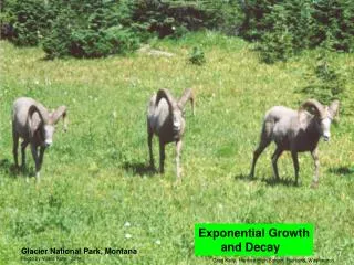
2. EXPONENTIAL GROWTH & DECAY • In many natural phenomena, • quantities grow or decay at a rate • proportional to their size.

3. EXPONENTIAL GROWTH & DECAY • Indeed, under ideal conditions—unlimited • environment, adequate nutrition, and • immunity to disease—the mathematical • model given by the equation f’(t) = kf(t) • predicts what actually happens fairly • accurately.

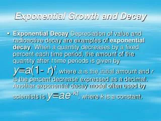
4. EXAMPLE • Another example occurs in nuclear • physics where the mass of a radioactive • substance decays at a rate proportional • to the mass.

5. EXAMPLE • In finance, the value of a savings • account with continuously compounded • interest increases at a rate proportional • to that value.

6. EXPONENTIAL GROWTH & DECAY Equation 1 • In general, if y(t) is the value of a quantity y • at time t and if the rate of change of y with • respect to t is proportional to its size y(t) • at any time, then • where k is a constant.

7. EXPONENTIAL GROWTH & DECAY • Equation 1 is sometimes called the law of • natural growth (if k > 0) or the law of natural • decay (if k < 0). • It is called a differential equation because • it involves an unknown function and its • derivative dy/dt.

8. EXPONENTIAL GROWTH & DECAY • It’s not hard to think of a solution of • Equation 1. • The equation asks us to find a function whose derivative is a constant multiple of itself. • We have met such functions in this chapter. • Any exponential function of the form y(t) = Cekt, where C is a constant, satisfies

9. EXPONENTIAL GROWTH & DECAY • We will see in Section 9.4 that any • function that satisfies dy/dt = ky must be • of the form y = Cekt. • To see the significance of the constant C, we observe that • Therefore, C is the initial value of the function.

10. EXPONENTIAL GROWTH & DECAY Theorem 2 • The only solutions of the differential • equation dy/dt = ky are the exponential • functions • y(t)= y(0)ekt

11. POPULATION GROWTH • What is the significance of • the proportionality constant k?

12. POPULATION GROWTH Example 1 • Use the fact that the world population was • 2,560 million in 1950 and 3,040 million in • 1960 to model the population in the second • half of the 20th century. (Assume the growth • rate is proportional to the population size.) • What is the relative growth rate? • Use the model to estimate the population in 1993 and to predict the population in 2020.

13. POPULATION GROWTH Example 1 • We measure the time t in years and let • t = 0 in 1950. • We measure the population P(t) in millions • of people. • Then, P(0) =2560 and P(10) =3040

14. POPULATION GROWTH Example 1 • Since we are assuming dP/dt = kP, • Theorem 2 gives:

15. POPULATION GROWTH Example 1 • The relative growth rate is about 1.7% • per year and the model is: • We estimate that the world population in 1993 was: • The model predicts that the population in 2020 will be:

16. POPULATION GROWTH Example 1 • The graph shows that the model is fairly • accurate to the end of the 20th century. • The dots represent the actual population.

17. POPULATION GROWTH Example 1 • So, the estimate for 1993 is quite reliable. • However, the prediction for 2020 is riskier.

18. Homework Pg. 239 # 1 - 4